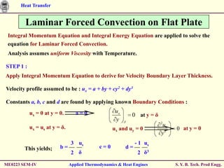
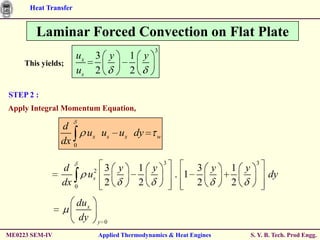
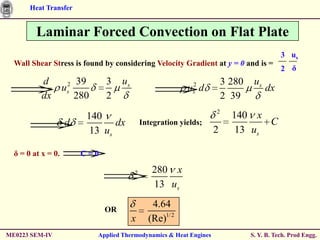
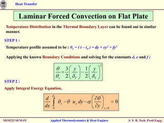
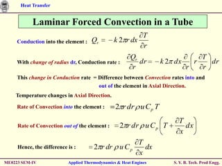
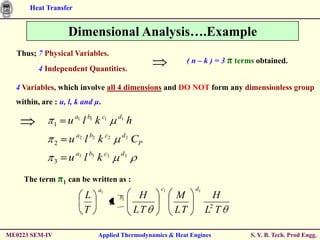
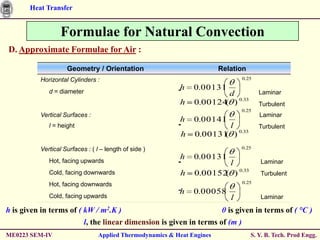
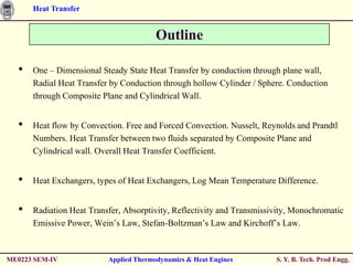
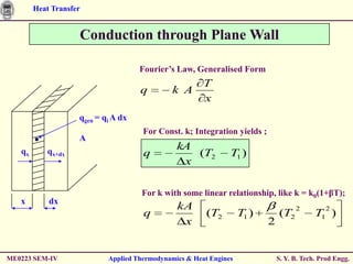
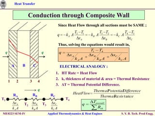
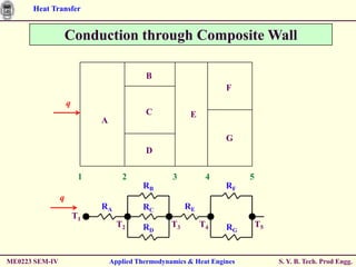
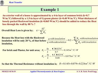
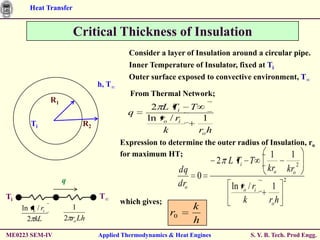
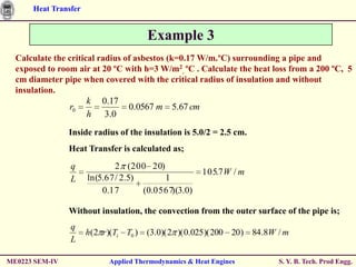
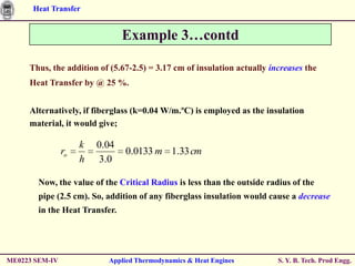
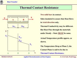
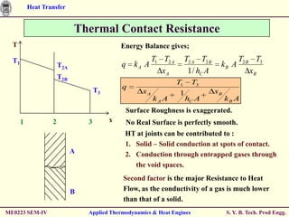
The document discusses heat transfer through conduction, convection and radiation. It covers key concepts like Fourier's law of heat conduction, thermal conductivity of solids, liquids and gases, one dimensional and radial heat conduction, and heat transfer through composite walls. It also provides examples of calculating heat transfer through plane and cylindrical walls, determining the required thickness of insulation, and calculating critical thickness of insulation.

1. Heat Transfer
Heat Transfer
Applied Thermodynamics & Heat Engines
S.Y. B. Tech.
ME0223 SEM - IV
Production Engineering
ME0223 SEM-IV Applied Thermodynamics & Heat Engines S. Y. B. Tech. Prod Engg.

2. Heat Transfer
Outline
• One – Dimensional Steady State Heat Transfer by conduction through plane wall,
Radial Heat Transfer by Conduction through hollow Cylinder / Sphere. Conduction
through Composite Plane and Cylindrical Wall.
• Heat flow by Convection. Free and Forced Convection. Nusselt, Reynolds and Prandtl
Numbers. Heat Transfer between two fluids separated by Composite Plane and
Cylindrical wall. Overall Heat Transfer Coefficient.
• Heat Exchangers, types of Heat Exchangers, Log Mean Temperature Difference.
• Radiation Heat Transfer, Absorptivity, Reflectivity and Transmissivity, Monochromatic
Emissive Power, Wein’s Law, Stefan-Boltzman’s Law and Kirchoff’s Law.
ME0223 SEM-IV Applied Thermodynamics & Heat Engines S. Y. B. Tech. Prod Engg.

3. Heat Transfer
Heat Transfer
HEAT TRANSFER is a science that seeks to predict the energy transfer that may
take place between material bodies, as a result of temperature difference.
Heat Transfer RATE is the desired objective of an analysis that points out the
difference between Heat Transfer and Thermodynamics.
Thermodynamics is dealt with equilibrium, and does not predict how fast the
change will take place.
Heat Transfer supplements the First and Second Laws of Thermodynamics, with
additional rules to analyse the Energy Transfer RATES.
ME0223 SEM-IV Applied Thermodynamics & Heat Engines S. Y. B. Tech. Prod Engg.

4. Heat Transfer
Conduction Heat Transfer
Fourier Law :
Heat Transfer (HT) Rate per unit cross – sectional (c/s) area is proportional
to the Temperature Gradient.
q T
A x
T
q k A
x
Q = HT Rate,
∂T/∂T = Temperature Gradient in the direction of Heat Flow.
k = Constant of Proportionality, known as THERMAL CONDUCTIVITY, (W/mºC)
NOTE : Negative sign is to indicate that Heat flows from High – Temperature to
Low – Temperature region, i.e. to satisfy Second Law of Thermodynamics.
ME0223 SEM-IV Applied Thermodynamics & Heat Engines S. Y. B. Tech. Prod Engg.

5. Heat Transfer
Conduction Heat Transfer
Heat Conduction through Plane Wall :
Generalised Case :
1. Temperature changes with time.
2. Internal Heat Sources.
Energy Balance gives;
qgen = qi A dx
Energy conducted in left face + Heat generated within element
A = Change in Internal Energy + Energy conducted out right face.
qx qx+dx T
Energy in left face = q kA
x
x
Energy generated within element = qi A dx
T
x dx Change in Internal Energy = cA dx
Energy out right face =
T T T
qx dx kA A k k dx
x x dx x x x
ME0223 SEM-IV Applied Thermodynamics & Heat Engines S. Y. B. Tech. Prod Engg.

6. Heat Transfer
Conduction Heat Transfer
Heat Conduction through Plane Wall :
Combining the terms;
T T T T
kA qi A dx cA dx A k k dx
x x x x
T T
qgen = qi A dx k qi c
x x
A This is One – Dimensional Heat Conduction Equation
qx qx+dx T T T T
kx ky kz qi c
x x y y z z
For Constant Thermal Conductivity, kx = ky = kz = k
2 2 2
x dx T T T qi 1 T
x2 y2 z2 k
Where, α = ( k / ρc ) is called Thermal Diffusivity. (m2/sec)
(↑) α ; (↑) the heat will diffuse through the material.
ME0223 SEM-IV Applied Thermodynamics & Heat Engines S. Y. B. Tech. Prod Engg.

7. Heat Transfer
Conduction Heat Transfer
2 2 2
T 1 T 1 T T qi 1 T
Heat Conduction through Cylinder :
r2 r r r2 2
z2 k
1 2 1 T 1 2
T qi 1 T
Heat Conduction through Sphere : rT sin
r r2 r 2 sin r 2 sin 2 2
k
Special Cases :
1. Steady State One – Dimensional (No Heat Generation) :
d 2T
0
dx2
2. Steady State One – Dimensional, Cylindrical co-ordinates (No Heat Generation) :
d 2T 1 dT
0
dr 2 r dr
3. Steady State One – Dimensional, with Heat Generation :
d 2T qi
0
dx2 k
ME0223 SEM-IV Applied Thermodynamics & Heat Engines S. Y. B. Tech. Prod Engg.

8. Heat Transfer
Thermal Conductivity
GAS : Kinetic Energy of the molecules of gas is transmitted from High – Temperature
region to that of Low – Temperature through continuous random motion,
colliding with one another and exchanging Energy as well as momentum.
LIQUIDS : Kinetic Energy is transmitted from High – Temperature region to that
of Low – Temperature by the same mechanism. BUT the situation is
more complex; as the molecules are closely spaced and molecular force
fields exert strong influence on the Energy exchange.
SOLIDS : (a) Free Electrons : Good Conductors have large number of free
electrons, which transfer electric charge as well as Thermal Energy.
Hence, are known as electron gas. EXCEPTION : Diamond !
(b) Lattice Vibrations : Vibrational Energy in lattice structure of the
material.
NOTE : Mode (a) is predominant than Mode (b).
ME0223 SEM-IV Applied Thermodynamics & Heat Engines S. Y. B. Tech. Prod Engg.

9. Heat Transfer
Thermal Conductivity
SOLIDS :
ME0223 SEM-IV Applied Thermodynamics & Heat Engines S. Y. B. Tech. Prod Engg.

10. Heat Transfer
Multilayer Insulation
Alternate Layers of Metal and Non-Metal
Metal having higher Reflectivity.
ME0223 SEM-IV Applied Thermodynamics & Heat Engines S. Y. B. Tech. Prod Engg.

11. Heat Transfer
Thermal Conductivity
LIQUIDS :
ME0223 SEM-IV Applied Thermodynamics & Heat Engines S. Y. B. Tech. Prod Engg.

12. Heat Transfer
Thermal Conductivity
GASES :
ME0223 SEM-IV Applied Thermodynamics & Heat Engines S. Y. B. Tech. Prod Engg.

13. Heat Transfer
Thermal Conductivity
Comparison :
ME0223 SEM-IV Applied Thermodynamics & Heat Engines S. Y. B. Tech. Prod Engg.

14. Heat Transfer
Conduction through Plane Wall
Fourier’s Law, Generalised Form
T
q k A
x
qgen = qi A dx
For Const. k; Integration yields ;
A
qx qx+dx
kA
q (T2 T1 )
x
For k with some linear relationship, like k = k0(1+βT);
x dx
kA 2 2
q (T2 T1 ) (T2 T1 )
x 2
ME0223 SEM-IV Applied Thermodynamics & Heat Engines S. Y. B. Tech. Prod Engg.

15. Heat Transfer
Conduction through Composite Wall
Since Heat Flow through all sections must be SAME ;
T2 T1 T3 T2 T4 T3
q kA A kB A kC A
xA xB xC
Thus, solving the equations would result in,
T1 T4
q q q
xA xB xC
kA A kB A kC A
A B C ELECTRICAL ANALOGY :
1. HT Rate = Heat Flow
2. k, thickness of material & area = Thermal Resistance
1 2 3 4
3. ΔT = Thermal Potential Difference.
q Therm alPotentialDifference
RA RB RC HeatFlow
Therm al sis tance
Re
T1 T4
xA xB xC Toverall
T2 T3 q
kA A kB A kC A Rth
ME0223 SEM-IV Applied Thermodynamics & Heat Engines S. Y. B. Tech. Prod Engg.

16. Heat Transfer
Conduction through Composite Wall
B
F
q
C E
A
G
D
1 2 3 4 5
RB RF
q
RA RC RE
T1
T2 RD T3 T4 RG T5
ME0223 SEM-IV Applied Thermodynamics & Heat Engines S. Y. B. Tech. Prod Engg.

17. Heat Transfer
Example 1
An exterior wall of a house is approximated by a 4-in layer of common brick (k=0.7
W/m.ºC) followed by a 1.5-in layer of Gypsum plaster (k=0.48 W/m.ºC). What thickness of
loosely packed Rockwool insulation (k=0.065 W/m.ºC) should be added to reduce the Heat
loss through the wall by 80 % ?
T
Overall Heat Loss is given by; q
Rth
Because the Heat loss with the Rockwool q with insulation Rth without insulation
insulation will be only 20 %, of that before 0.2
q withoutinsulation Rth with insulation
insulation,
x 4 0.0254
For brick and Plaster, for unit area; Rb 0.145 m 2 . C / W
k 0.7
x 1.5 0.0254
Rp 0.079 m 2 . C / W
k 0.48
2
So that the Thermal Resistance without insulation is; R 0.145 0.079 0.224 m . C / W
ME0223 SEM-IV Applied Thermodynamics & Heat Engines S. Y. B. Tech. Prod Engg.

18. Heat Transfer
Example 1…contd
0.224
Now; R with Insulation 1.122 m 2 . C / W
0.2
This is the SUM of the previous value and the Resistance for the Rockwool.
1.122 0.224 Rrw
x x
Rrw 0.898
k 0.065
xrw 0.0584m 2.30 in …ANS
ME0223 SEM-IV Applied Thermodynamics & Heat Engines S. Y. B. Tech. Prod Engg.

19. Heat Transfer
Conduction through Radial Systems
Cylinder with;
1. Inside Radius, ri.
2. Outside Radius, ro.
3. Length, L
4. Temperature Gradient, Ti-To
q
5. L >> r; → Heat Flow in Radial direction only.
dr
ro
ri r Area for Heat Flow;
Ar = 2πrL
T T
Fourier’s Law will be, q k Ar 2 krL
r r
q Boundary Conditions :
RA T = Ti at r = ri
Ti To
T = To at r = ro
ln ro / ri 2 k L Ti To
Rth q
2 kL Solution to the Equation is;
ln ro / ri
ME0223 SEM-IV Applied Thermodynamics & Heat Engines S. Y. B. Tech. Prod Engg.

20. Heat Transfer
Conduction through Radial Systems
q Thermal Resistance is,
T4 ln ro / ri
Rth
T3 2 kL
R1 T2
For Composite Cylinder;
T1 R2
2 L T1 T4
A q
R3 ln r2 / r1 / k A ln r3 / r2 / k B ln r4 / r3 / k B
B
C R4
For Spheres;
q
RA RB RC 4 k Ti To
T1 T4 q
1 1
ln r2 / r1 T2 ln r3 / r2 T3 ln r4 / r3 ri ro
2 kAL 2 kB L 2 kC L
ME0223 SEM-IV Applied Thermodynamics & Heat Engines S. Y. B. Tech. Prod Engg.

21. Heat Transfer
Example 2
A thick-walled tube of stainless steel (18% Cr, 8% Ni, k=19 W/m.ºC) with 2 cm inner
diameter (ID) and 4 cm outer diameter (OD) is covered with a 3 cm layer of asbestos
insulation (k=0.2 W/m.ºC). If the inside wall temperature of the pipe is maintained at
600 ºC, calculate the heat loss per meter of length and the tube-insulation interface
temperature.
Heat flow is given by;
q
q 2 (T1 T3 ) 2 (600 100)
T3=100 ºC 680W / m
L ln r2 / r1 / kS ln r3 / r2 / k A ln 2 / 1 / 19 ln 5 / 2 / 0.2
This Heat Flow is used to calculate the tube-insulation
R1 T2
interface temperature as;
R2 q (T2 T3 )
T1=600 ºC 680W / m
L ln r3 / r2 / 2 k A
R3
T2 = 595.8 ºC…ANS
Stainless Steel
Asbestos
S. Y. B. Tech. Prod Engg.

22. Heat Transfer
Critical Thickness of Insulation
Consider a layer of Insulation around a circular pipe.
Inner Temperature of Insulator, fixed at Ti
Outer surface exposed to convective environment, T∞
h, T∞
From Thermal Network;
R1
2 L Ti T
q
ln ro / ri 1
Ti R2
k ro h
Expression to determine the outer radius of Insulation, ro
for maximum HT; 1 1
2 L Ti T 2
dq kro kro
q
0 2
dro ln ro / ri 1
Ti T∞ k ro h
which gives;
ln ro / ri 1 k
r0
2 kL 2 ro Lh h
ME0223 SEM-IV Applied Thermodynamics & Heat Engines S. Y. B. Tech. Prod Engg.

23. Heat Transfer
Example 3
Calculate the critical radius of asbestos (k=0.17 W/m.ºC) surrounding a pipe and
exposed to room air at 20 ºC with h=3 W/m2. ºC . Calculate the heat loss from a 200 ºC, 5
cm diameter pipe when covered with the critical radius of insulation and without
insulation.
k 0.17
r0 0.0567 m 5.67 cm
h 3.0
Inside radius of the insulation is 5.0/2 = 2.5 cm.
Heat Transfer is calculated as;
q 2 (200 20)
105.7 W / m
L ln(5.67 / 2.5) 1
0.17 (0.0567)(3.0)
Without insulation, the convection from the outer surface of the pipe is;
q
h(2 r )(Ti T0 ) (3.0)( 2 )( 0.025 )( 200 20) 84.8W / m
L
ME0223 SEM-IV Applied Thermodynamics & Heat Engines S. Y. B. Tech. Prod Engg.

24. Heat Transfer
Example 3…contd
Thus, the addition of (5.67-2.5) = 3.17 cm of insulation actually increases the
Heat Transfer by @ 25 %.
Alternatively, if fiberglass (k=0.04 W/m.ºC) is employed as the insulation
material, it would give;
k 0.04
ro 0.0133 m 1.33 cm
h 3.0
Now, the value of the Critical Radius is less than the outside radius of the
pipe (2.5 cm). So, addition of any fiberglass insulation would cause a decrease
in the Heat Transfer.
ME0223 SEM-IV Applied Thermodynamics & Heat Engines S. Y. B. Tech. Prod Engg.

25. Heat Transfer
Thermal Contact Resistance
Two solid bars in contact.
q q
A B Sides insulated to assure that Heat flows
in Axial direction only.
ΔxA ΔxB Thermal Conductivity may be different.
But Heat Flux through the materials
T
under Steady – State MUST be same.
T1
T2A
Actual Temperature profile approx. as
T2B
shown.
T3
The Temperature Drop at Plane 2, the
Contact Plane is said to be due to
1 2 3 x Thermal Contact Resistance.
ME0223 SEM-IV Applied Thermodynamics & Heat Engines S. Y. B. Tech. Prod Engg.

26. Heat Transfer
Thermal Contact Resistance
T Energy Balance gives;
T1 T1 T2 A T2 A T2 B T2 B T3
T2A q kA A kB A
xA 1 / hC A xB
T2B
T1 T3
q
T3 xA 1 xB
kA A hC A kB A
Surface Roughness is exaggerated.
1 2 3 x No Real Surface is perfectly smooth.
HT at joints can be contributed to :
1. Solid – Solid conduction at spots of contact.
A 2. Conduction through entrapped gases through
the void spaces.
Second factor is the major Resistance to Heat
B Flow, as the conductivity of a gas is much lower
than that of a solid.
ME0223 SEM-IV Applied Thermodynamics & Heat Engines S. Y. B. Tech. Prod Engg.

27. Heat Transfer
Thermal Contact Resistance
Designating;
1. Contact Area, Ac
A 2. Void Area, Av
3. Thickness of Void Space, Lg
4. Thermal Conductivity of the Fluid in Void space, kf
T2 A T2 B T2 A T2 B T2 A T2 B
q k f Av
B Lg / 2k A AC Lg / 2k B AC Lg 1 / hC A
Total C/s. Area of the bars is A.
Solving for hc;
T2A 1 AC 2k A k B Av
hC kf
Lg Lg A k A kB A
T2B Most usually, AIR is the fluid in void spaces.
Hence, kf is very small compared to kA and kB.
ME0223 SEM-IV Applied Thermodynamics & Heat Engines S. Y. B. Tech. Prod Engg.

28. Heat Transfer
Example 4
Two 3.0 cm diameter 304 stainless steel bars, 10 cm long have ground surface and are
exposed to air with a surface roughness of about 1 μm. If the surfaces are pressed
together with a pressure of 50 atm and the two-bar combination is exposed to an overall
temperature difference of 100 ºC, calculate the axial Heat Flow and Temperature Drop
across the contact surface. Take 1/hc=5.28 X 10-4 m2.ºC/W.
The overall Heat Flow is subject to three resistances,
1. One Conducting Resistance for each bar
2. Contact Resistance.
x (0.1)(4)
For the bars; Rth 8.679 C / W
kA (16.3) (3 X 100 2 ) 2
1 (5.28X 10 4 )(4)
Contact Resistance; RC 0.747 C / W
hC A (3 X 10 2 ) 2
Total Thermal Resistance; Rth (2)(3.679) 0.747 8.105 C / W
ME0223 SEM-IV Applied Thermodynamics & Heat Engines S. Y. B. Tech. Prod Engg.

29. Heat Transfer
Example 4…contd
T 100
Overall Heat Flow is; q 12.338 W …ANS
Rth 8.105
Temperature Drop across the contact is found by taking the ratio of the Contact
Resistance to the Total Resistance.
RC (0.747)
TC T (100) 6.0544 C …ANS
Rth 12.338
i.e. 6 % of the total resistance.
ME0223 SEM-IV Applied Thermodynamics & Heat Engines S. Y. B. Tech. Prod Engg.

30. Heat Transfer
Radiation Heat Transfer
Physical Interpretation :
Thermal Radiation is the electromagnetic radiation as result of its temperature.
There are many types of electromagnetic radiations, Thermal Radiation is one of them.
Regardless of the type, electromagnetic radiation is propagated at the speed of light,
3 X 108 m/sec. This speed is the product of wavelength and frequency of the radiation.
c = Speed of light
c=λυ λ = Wavelength
υ = Frequency
NOTE : Unit of λ may be cm, A˚ or μm.
ME0223 SEM-IV Applied Thermodynamics & Heat Engines S. Y. B. Tech. Prod Engg.

31. Heat Transfer
Radiation Heat Transfer
Thermal
Radiation
log λ, m 1 μm 1 A˚
3 2 1 0 -1 -2 -3 -4 -5 -6 -7 -8 -9 -10 -11 -12
X-Rays
Radio
Waves Infrared Ultraviolet γ-Rays
Visible
Thermal Radiation → 0.1 – 100 μm.
Visible Light Portion → 0.35 – 0.75 μm.
S. Y. B. Tech. Prod Engg.

32. Heat Transfer
Radiation Heat Transfer
Physical Interpretation :
Propagation of Thermal radiation takes place in the form of discrete quanta.
Each quantum having energy; E = hυ
h is Planck’s Constant, given by;
h = 6.625 X 10-34 J.sec
A very basic physical picture of the Radiation propagation →
Considering each quantum as a particle having Energy, Mass and momentum.
E = mc2 = hυ
m = hυ
c2
& Momentum = c (hυ) = hυ
c2 c
ME0223 SEM-IV Applied Thermodynamics & Heat Engines S. Y. B. Tech. Prod Engg.

33. Heat Transfer
Stefan – Boltzmann Law
Applying the principles of Quantum-Statistical Thermodynamics;
Energy Density per unit volume per unit wavelength; 8 hc 5
u
e hc / kT 1
Where, k is Boltzmann’s Constant; 1.38066 X 10-23 J/molecule.K
When Energy Density is integrated over all wavelengths;
Total Energy emitted is proportional to the fourth power of absolute temperature.
Eb = ζT4
Equation is known as Stefan – Boltzmann Law.
Eb = Energy radiated per unit time per unit area by the ideal radiator, W/m2
ζ = Stefan – Boltzmann Constant; 5.667 X 10-8 W/m2.K4
ME0223 SEM-IV Applied Thermodynamics & Heat Engines S. Y. B. Tech. Prod Engg.

34. Heat Transfer
Stefan – Boltzmann Law
Subscript b in this equation → Radiation from a Blackbody.
Materials which obey this Law appear black to the eye, as they do not reflect any
radiation.
Thus, a Blackbody is a body which absorbs all the radiations incident upon it.
Eb is known as the Emissive Power of the Blackbody.
i.e. Energy radiated per unit time per unit area.
Eb = ζT4 qemitted = ζ.A.T4
NOTE : “Blackness” of a surface to Thermal Radiation can be quite deceiving.
e.g. Lamp-black…..and Ice….!!!
ME0223 SEM-IV Applied Thermodynamics & Heat Engines S. Y. B. Tech. Prod Engg.

35. Heat Transfer
Radiation Properties
Radiant Energy incident on a surface;
(a) Part is Reflected,
(b) Part is Absorbed,
(c) Part is Transmitted.
Incident
Radiation Reflection Reflected Energy
Reflectivity = ρ =
Incident Energy
Absorbed Energy
Absorption Absorptivity = α =
Incident Energy
Transmitted Energy
Transmissivity = η =
Transmission Incident Energy
ρ+α+η=1
NOTE : Most solids do not transmit Thermal Radiations. → ρ+α=1
ME0223 SEM-IV Applied Thermodynamics & Heat Engines S. Y. B. Tech. Prod Engg.

36. Heat Transfer
Radiation Properties
Types of Reflection :
1. Angle of Incidence = Angle of Reflection → Specular Reflection
2. Incident beam distributed uniformly in all directions → Diffuse Reflection
Source
Source
θ1 θ2
Specular Reflection Diffuse Reflection
Offers the Mirror Image to the Observer
ME0223 SEM-IV Applied Thermodynamics & Heat Engines S. Y. B. Tech. Prod Engg.

37. Heat Transfer
Radiation Properties
No REAL surface cab be perfectly Specular or Diffuse.
Ordinary mirror → Specular for visible region; but may not be in complete spectrum
of Thermal Radiation.
Rough surface exhibits the Diffused behaviour.
Polished surface exhibits the Specular behaviour.
ME0223 SEM-IV Applied Thermodynamics & Heat Engines S. Y. B. Tech. Prod Engg.

38. Heat Transfer
Kirchhoff’s Law
Assume perfect Black enclosure.
Radiant flux incident is qi W/m2.
A Sample body placed inside Enclosure, in
Black Enclosure
Thermal Equilibrium with it.
EA qiAα
Sample
Energy Absorbed by the Sample = Energy emitted.
i.e. E A = qi A α …(I)
Replacing the Sample Body with a Blackbody;
Eb A = qi A (1) …(II)
Dividing (I) by (II);
E / Eb = α
ME0223 SEM-IV Applied Thermodynamics & Heat Engines S. Y. B. Tech. Prod Engg.

39. Heat Transfer
Kirchhoff’s Law
Ratio of Emissive Power of a body
Black Enclosure
to that of a Perfectly Black body, at
the same temperature is known as
EA qiAα
Sample Emissivity, ε of the body.
ε = E / Eb
Thus;
ε=α
This is known as Kirchhoff’s Identity.
ME0223 SEM-IV Applied Thermodynamics & Heat Engines S. Y. B. Tech. Prod Engg.

40. Heat Transfer
Gray Body
Gray Body can be defined as the body whose Monochromatic Emissivity, ελ is
independent of wavelength.
Monochromatic Emissivity is defined as the ratio of Monochromatic Emissive
Power of the body to that of a Blackbody at the SAME wavelength and
temperature.
ελ = Eλ / Ebλ
Total Emissivity of the body is related to the Monochromatic Emissivity as;
E Eb d And Eb Eb d T4
0 0
Eb d
Thus, E 0
EB T4
ME0223 SEM-IV Applied Thermodynamics & Heat Engines S. Y. B. Tech. Prod Engg.

41. Heat Transfer
Gray Body
When the GRAY BODY condition is applied,
ελ = ε
A functional relation for Ebλ was derived by Planck by introducing the concept of
QUANTUM in Electromagnetic Theory.
The derivation is by Statistical Thermodynamics.
u c
By this theory, Ebλ is related to the Energy Density by; Eb
4
5
C1
Eb
Where, λ = Wavelength, μm e C2 / T
1
T = Temperature, K
C1 = 3.743 X 108 ,W.μm/m2
C2 = 1.4387 X 104, μm.K
ME0223 SEM-IV Applied Thermodynamics & Heat Engines S. Y. B. Tech. Prod Engg.

42. Heat Transfer
Wien’s Displacement Law
A plot of Ebλ as a function of T and λ.
Peak of the curve is shifted to
SHORTER Wavelengths at
HIGHER Temperatures.
Points of the curve are related by;
λmax T = 2897.6 μm.K
This is known as Wien’s
Displacement Law.
ME0223 SEM-IV Applied Thermodynamics & Heat Engines S. Y. B. Tech. Prod Engg.

43. Heat Transfer
Wien’s Displacement Law
Shift in the maximum point of the Radiation Curve helps to explain the change in colour
of a body as it is heated.
Band of wavelengths visible to the eye lies between 0.3 – 0.7 μm.
Very small portion of the radiant energy spectrum at low temperatures is visible to eye.
As the body is heated, maximum intensity shifts to shorter wavelengths.
Accordingly, first visible sight of increase in temperature of a body is DARK RED
colour.
Further heating yields BRIGHT RED colour.
Then BRIGHT YELLOW.
And, finally WHITE…!!
Material also looks brighter at higher temperatures, as large portion of the total
radiation falls within the visible range.
ME0223 SEM-IV Applied Thermodynamics & Heat Engines S. Y. B. Tech. Prod Engg.

44. Heat Transfer
Radiation Heat Transfer
General interest in amount of Energy radiated from a Blackbody in a certain
specified Wavelength range.
Eb d
Eb 0
The fraction of Total Energy Radiated between 0 to λ is given by; 0
Eb 0
Eb d
Eb C1 0
Diving both sides by T5; 5
T5 T e C2 / T
1
This ratio is standardized in Graph as well as Tabular forms; with parameters as;
1. λT
2. Ebλ / T5
3. Eb 0-λT / ζT4
ME0223 SEM-IV Applied Thermodynamics & Heat Engines S. Y. B. Tech. Prod Engg.

45. Heat Transfer
Radiation Heat Transfer
If the Radiant Energy between Wavelengths λ1 and λ2 are desired;
Eb 0 Eb 0
Eb Eb 0 2 1
1 2
Eb 0 Eb 0
NOTE : Eb 0-∞ is the Total Radiation emitted over all Wavelengths = ζT4
ME0223 SEM-IV Applied Thermodynamics & Heat Engines S. Y. B. Tech. Prod Engg.

46. Heat Transfer
Radiation Heat Transfer
EXAMPLE :
Solar Radiation has a spectrum, approx. to that of a Blackbody at 5800 K.
Ordinary window glass transmits Radiation to about 2.5 μm.
From the Table for Radiation Function, λT = (2.5)(5800) = 14,500 μm.K
The fraction of then Solar Spectrum is about 0.97.
Thus, the regular glass transmits most of the Radiation incident upon it.
On the other hand, the room Radiation at 300 K has λT = (2.5)(300) = 750 μm.K
Radiation Fraction corresponding to this value is 0.001 per cent.
Thus, the ordinary glass essentially TRANSPARENT to Visible light, is almost OPAQUE
for Thermal Radiation at room temperature.
ME0223 SEM-IV Applied Thermodynamics & Heat Engines S. Y. B. Tech. Prod Engg.

47. Heat Transfer
Heat Exchangers
Overall Heat Transfer Coefficient :
Heat Transfer is expressed as;
TA kA
q h1 A (TA T1 ) (T1 T2 ) h2 A (T2 TB )
h2 x
Applying the Thermal Resistance;
Fluid B
T1 (TA TB )
q
q T2 (1 / h1 A) ( x / kA) (1 / h2 A)
Overall Heat Transfer by combined
Fluid A
Conduction + Convection is expressed in
h1
TB terms of Overall Heat Transfer Coefficient ,
U, defined as;
q
RA RB RC q = U A ΔToverall
TA TB
1 x 1 1
T1 T2 U
h1 A kA h2 A (1 / h1 ) ( x / k ) (1 / h2 )
ME0223 SEM-IV Applied Thermodynamics & Heat Engines S. Y. B. Tech. Prod Engg.

48. Heat Transfer
Heat Exchangers
Overall Heat Transfer Coefficient :
Hollow Cylinder exposed to
Fluid B in
Convective environment on its inner
and outer surfaces.
Fluid A in
Area for Convection is NOT same for
both fluids.
→ ID and thickness of the inner tube.
q Overall Heat Transfer would be;
RA RB RC
TA TB (TA TB )
1 1 q
Ti ln (ro / ri ) To 1 ln (r0 / ri ) 1
hi Ai 2 kL ho Ao
hi Ai 2 kL ho Ao
ME0223 SEM-IV Applied Thermodynamics & Heat Engines S. Y. B. Tech. Prod Engg.

49. Heat Transfer
Heat Exchangers
Overall Heat Transfer Coefficient :
Overall Heat Transfer Coefficient can be based on either INNER side or OUTER area
of the tube.
1
Based in INNER Area; Ui
1 Ai ln (r0 / ri ) Ai 1
hi 2 kL Ao ho
1
Based in OUTER Area; Uo
Ao 1 Ao ln (r0 / ri ) 1
Ai hi 2 kL ho
1
In general, for either Plane Wall or Cylinder, UA
Rth
ME0223 SEM-IV Applied Thermodynamics & Heat Engines S. Y. B. Tech. Prod Engg.

50. Heat Transfer
Example 5
Water flows at 50 °C inside a 2.5 cm inside diameter tube such that hi = 3500 W/m2.°C.
The tube has a wall thickness of 0.8 mm with thermal conductivity of 16 W/m.°C. The
outside of the tube loses heat by free convection with ho = 7.6 W/m2.°C.Calculate the
overall heat transfer coefficient and heat air at 20 °C.
3 Resistances in series.
L = 1.0 mtr, di = 0.025 mtr and do = 0.025 + (2)(0.008) mtr = 0.0266 mtr.
1 1
Ri 0.00364 C / W
hi Ai (3500 (0.025)(1.0)
)
ln (d o / di ) ln (0.0266/ 0.025)
Rt 0.00062 C / W
2 kL 2 (16)(1.0)
1 1
Ro 1.575 C / W
ho Ao (7.6) (0.0266 1.0)
)(
ME0223 SEM-IV Applied Thermodynamics & Heat Engines S. Y. B. Tech. Prod Engg.

51. Heat Transfer
Example 5….contd
This clearly states that the controlling resistance for the Overall Heat Transfer
Coefficient is Outside Convection Resistance.
Hence, the Overall Heat Transfer Coefficient is based on Outside Tube Area.
Toverall
q U 0 Ao T
Rth
1 1
U0
A0 Rth (0.0266 1.0) 0.00364 0.00062 1.575
)(
7.577 W / m 2 . C ….ANS
Heat Transfer is obtained by;
q Uo Ao T (7.577) (0.0266 1.0)(50 20) 19 W ….ANS
)(
ME0223 SEM-IV Applied Thermodynamics & Heat Engines S. Y. B. Tech. Prod Engg.

52. Heat Transfer
Heat Exchangers
Fouling Factor :
After a period, the performance of the Heat Exchanger gets degraded as;
1. HT surface may become coated with various deposits.
2. HT surface may get corroded due to interaction between fluid and material.
This coating offers additional Resistance to the Heat Flow.
Performance Degradation effect is presented by introducing Fouling Factor or
Fouling Resistance, Rf.
1 1
Fouling Factor, Rf is defined as; Rf
U dirty U clean
ME0223 SEM-IV Applied Thermodynamics & Heat Engines S. Y. B. Tech. Prod Engg.

53. Heat Transfer
Types of Heat Exchangers
Shell-And-Tube Heat Exchanger :
ME0223 SEM-IV Applied Thermodynamics & Heat Engines S. Y. B. Tech. Prod Engg.

54. Heat Transfer
Types of Heat Exchangers
Shell-And-Tube Heat Exchanger :
ME0223 SEM-IV Applied Thermodynamics & Heat Engines S. Y. B. Tech. Prod Engg.

55. Heat Transfer
Types of Heat Exchangers
Shell-And-Tube Heat Exchanger :
ME0223 SEM-IV Applied Thermodynamics & Heat Engines S. Y. B. Tech. Prod Engg.

56. Heat Transfer
Types of Heat Exchangers
Shell-And-Tube Heat Exchanger :
ME0223 SEM-IV Applied Thermodynamics & Heat Engines S. Y. B. Tech. Prod Engg.

57. Heat Transfer
Types of Heat Exchangers
Miniature / Compact Heat Exchanger :
ME0223 SEM-IV Applied Thermodynamics & Heat Engines S. Y. B. Tech. Prod Engg.

58. Heat Transfer
Types of Heat Exchangers
Cross-Flow Heat Exchanger :
ME0223 SEM-IV Applied Thermodynamics & Heat Engines S. Y. B. Tech. Prod Engg.

59. Heat Transfer
Types of Heat Exchangers
Cross-Flow Heat Exchanger :
S. Y. B. Tech. Prod Engg.

60. Heat Transfer
Log Mean Temperature Difference
TEMPERATURE PROFILES :
T
T
Th1 Hot Fluid
Th1 Hot Fluid
dq
dq
Th Tc1 Th
Th2 Th2
Tc
Tc Tc2
dA
dA
Cold Fluid Cold Fluid Tc2
Tc1
A A
1 2 1 2
Parallel Flow Counter Flow
ME0223 SEM-IV Applied Thermodynamics & Heat Engines S. Y. B. Tech. Prod Engg.

61. Heat Transfer
Log Mean Temperature Difference
q = U A ΔTm
T
dq = U dA (Th-Tc) U = Overall Heat Transfer Coefficient.
Hot Fluid A = Surface Area for Heat Transfer
Th1
dq consistent with definition of U.
Th ΔTm = Suitable Mean Temperature
Th2
Difference across Heat Exchanger.
Tc Tc2
As can be seen, the Temperature
dA Difference between the Hot and Cold
Tc1 Cold Fluid
fluids vary between Inlet and Outlet.
A Average Heat Transfer Area for the
1 2
above equation is required.
ME0223 SEM-IV Applied Thermodynamics & Heat Engines S. Y. B. Tech. Prod Engg.

62. Heat Transfer
Log Mean Temperature Difference
Heat transferred through elemental area dA;
T
dq = U dA (Th-Tc) dq mh Ch dTh mc Cc dTc
Th1 Hot Fluid dq U dA(Th Tc )
dq
Th dq dq
Th2 dTh And; dTc
m h Ch m c Cc
Tc Tc2
dA 1 1
Cold Fluid dTh dTc d (Th Tc ) dq
Tc1
m h Ch m c Cc
Solving for dq;
A
1 2 d (Th Tc ) 1 1
U dA
Th Tc m h Ch m c Cc
ME0223 SEM-IV Applied Thermodynamics & Heat Engines S. Y. B. Tech. Prod Engg.

63. Heat Transfer
Log Mean Temperature Difference
Equation can be integrated between
conditions 1 and 2 to yield;
T
dq = U dA (Th-Tc)
(Th 2 Tc 2 ) 1 1
ln UA
Th1 Hot Fluid (Th1 Tc1 ) m h Ch m c Cc
dq
Th Again;
Th2 q q
m h Ch & mc Cc
(Th1 Th 2 ) (Tc 2 Tc1 )
Tc Tc2
This substitution gives;
dA
Tc1 Cold Fluid (Th 2 Tc 2 ) (Th1 Tc1 )
q UA
ln (Th 2 Tc 2 ) /(Th1 Tc1 )
A
1 2 (Th 2 Tc 2 ) (Th1 Tc1 )
OR; Tm
ln (Th 2 Tc 2 ) /(Th1 Tc1 )
ME0223 SEM-IV Applied Thermodynamics & Heat Engines S. Y. B. Tech. Prod Engg.

64. Heat Transfer
Log Mean Temperature Difference
This Temperature Difference, ΔTm , is known as Log Mean Temperature Difference.
Tone end of HE Tother end of HE
LMTD
natural log Ratio of both Ts
Main Assumption :
1. Specific Heats (Cc and Ch) of fluids do not vary with Temperatures.
2. Convective HT Coefficients (h) are constant throughout the Heat Exchanger.
Serious concerns for validity due to : 1. Entrance Effects.
2. Fluid Viscosity.
3. Change in Th. Conductivity.
ME0223 SEM-IV Applied Thermodynamics & Heat Engines S. Y. B. Tech. Prod Engg.

65. Heat Transfer
Log Mean Temperature Difference
ME0223 SEM-IV Applied Thermodynamics & Heat Engines S. Y. B. Tech. Prod Engg.

66. Heat Transfer
Log Mean Temperature Difference
ME0223 SEM-IV Applied Thermodynamics & Heat Engines S. Y. B. Tech. Prod Engg.

67. Heat Transfer
Log Mean Temperature Difference
ME0223 SEM-IV Applied Thermodynamics & Heat Engines S. Y. B. Tech. Prod Engg.

68. Heat Transfer
Log Mean Temperature Difference
ME0223 SEM-IV Applied Thermodynamics & Heat Engines S. Y. B. Tech. Prod Engg.

69. Heat Transfer
Example 6
Water at the rate of 68 kg/min is heated from 35 to 75 °C by an oil having specific
heat of 1.9 kJ/kg.°C. The fluids are used in a counterflow double-pipe heat exchanger,
and the oil enters in the exchanger at 110 °C and leaves at 75 °C. The overall heat
transfer coefficient is 320 W/m2.°C. Calculate the heat exchanger area.
Total Heat Transfer is calculated by Energy absorbed by water;
q m w Cw Tw (68)(4.18)(75 35) 11.37 MJ / min 189.5 kW
Since all fluid temperatures are known, LMTD T
can be calculated.
110 °C Hot Fluid Th
(Th 2 Tc 2 ) (Th1 Tc1 ) dq
Tm
ln (Th 2 Tc 2 ) /(Th1 Tc1 ) 75 °C 75 °C
(75 35) (110 75) Tc
37.44 C
ln (75 35) /(110 75)
dA 35 °C
And; q U A Tm Yields;
q 189.5 X 103 Cold Fluid
A 15.82 m2….ANS A
U Tm (320)(37.44) 1 2
ME0223 SEM-IV Applied Thermodynamics & Heat Engines S. Y. B. Tech. Prod Engg.

70. Heat Transfer
Example 7
In stead of double-pipe heat exchanger, of Example 6, it is desired to use a shell-and-
tube heat exchanger with water making one shell pass and oil making two tube
passes. Calculate the heat exchanger area assuming other conditions same.
T1 = 35 °C T2 = 75 °C t1 = 110 °C t2 = 75 °C
t2 t1 75 110
P 0.467
T1 t1 35 110
T1 T2 35 75
R 1.143
t2 t1 75 110
Correction Factor from Chart = 0.8
q U A F Tm yields;
q 189.5 X 103
A 19.53 m2 ….ANS
U F Tm (320)(0.8)(37.44)
ME0223 SEM-IV Applied Thermodynamics & Heat Engines S. Y. B. Tech. Prod Engg.

71. Heat Transfer
Effectiveness-NTU Method
LMTD approach is suitable when both the inlet and outlet temperatures are known,
or can be easily computed.
However, when the temperatures are to be evaluated by an iterative method, analysis
becomes quite complicated as it involves the Logarithmic function.
In this case, the method of analysis is based on the Effectiveness of the Heat
Exchanger in transferring the given amount of Heat.
Effectiveness of the Heat Exchanger is defined as;
Actual Heat Transfer
Effectiveness
Maxim umPossible Heat Transfer
Actual Heat Transfer is calculated by;
1. Energy lost by HOT fluid. OR
2. Energy gained by COLD fluid.
ME0223 SEM-IV Applied Thermodynamics & Heat Engines S. Y. B. Tech. Prod Engg.

72. Heat Transfer
Effectiveness-NTU Method
For Parallel-Flow Heat Exchanger; q mh Cph (Th1 Th 2 ) mc Cpc (Tc 2 Tc1 )
For Counter-Flow Heat Exchanger; q mh Cph (Th1 Th 2 ) mc Cpc (Tc1 Tc 2 )
Maximum possible Heat Transfer Maximum possible Temperature Difference
Difference in INLET Temperatures
of Hot and Cold fluids.
Maximum Temperature Difference Minimum (m C ) value.
Thus;
Maximum Heat Transfer is given by; qmax (m Cp) min (Thinlet Tcinlet )
The ( m Cp )fluid may be Hot or Cold, depending on their respective mass flow rates
and Specific Heats.
ME0223 SEM-IV Applied Thermodynamics & Heat Engines S. Y. B. Tech. Prod Engg.

73. Heat Transfer
Effectiveness-NTU Method
mh Cph (Th1 Th 2 ) Th1 Th 2
h
mh Cph (Th1 Tc1 ) Th1 Tc1
For Parallel-Flow Heat Exchanger;
mc Cpc (Tc 2 Tc1 ) Tc 2 Tc1
c
mc Cpc (Th1 Tc1 ) Th1 Tc1
mh Cph (Th1 Th 2 ) Th1 Th 2
h
mh Cph (Th1 Tc 2 ) Th1 Tc 2
For Counter-Flow Heat Exchanger;
mc Cpc (Tc1 Tc 2 ) Tc1 Tc 2
c
mc Cpc (Th1 Tc 2 ) Th1 Tc 2
ME0223 SEM-IV Applied Thermodynamics & Heat Engines S. Y. B. Tech. Prod Engg.

74. Heat Transfer
Effectiveness-NTU Method
Effectiveness, ε, can be derived in a different way;
For Parallel-Flow Heat Exchanger; ln (Th 2 Tc 2 ) UA
1 1
(Th1 Tc1 ) m h Cph m c Cpc
T
dq = U dA (Th-Tc)
UA m c Cpc
Th1 Hot Fluid 1
dq m c Cpc m h Cph
Th
Th2
OR (Th 2 Tc 2 ) UA m c Cpc
exp 1
Tc2 (Th1 Tc1 ) m c Cpc m h Cph
Tc
dA
Cold Fluid If Cold fluid is min ( m Cp ) fluid;
Tc1
Tc 2 Tc1
A c
Th1 Tc1
1 2
ME0223 SEM-IV Applied Thermodynamics & Heat Engines S. Y. B. Tech. Prod Engg.

75. Heat Transfer
Effectiveness-NTU Method
We know; dq m h Cph dTh mc Cpc dTc
mc Cpc
mh Cph (Th1 Th 2 ) mc Cpc (Tc 2 Tc1 ) Th 2 Th1 (Tc1 Tc 2 )
mh Cph
This yields; (Th 2 Tc 2 ) Th1 (mc Cpc / m h Cph )(Tc1 Tc 2 ) Tc 2
(Th1 Tc1 ) (Th1 Tc1 )
(Th1 Tc1 ) (m c Cpc / m h Cph )(Tc1 Tc 2 ) (Tc1 Tc 2 ) m c Cpc
1 1 c
(Th1 Tc1 ) m h Cph
1 exp UA / m c Cpc 1 (m c Cpc / m h Cph )
c
1 (m c Cpc / m h Cph )
ME0223 SEM-IV Applied Thermodynamics & Heat Engines S. Y. B. Tech. Prod Engg.

76. Heat Transfer
Effectiveness-NTU Method
It can be shown that the SAME expression results if Hot fluid is min ( m Cp ) fluid;
EXCEPT that (mc Cpc )and (mh Cp h ) are interchanged.
1 exp UA / Cmin 1 Cmin / Cmax
In a General Form; parallel
1 Cmin / Cmax
where, C = (m C ) ; defined as CAPACITY RATE.
Similar analysis for Counter-Flow Heat Exchanger yields;
1 exp UA / Cmin 1 Cmin / Cmax
counter
1 (Cmin / Cmax ) exp UA / Cmin 1 Cmin / Cmax
The group of terms, (UA/Cmin ) is known as Number of Transfer Units (NTU).
This is so, since it is the indication of the size of the Heat Exchanger.
ME0223 SEM-IV Applied Thermodynamics & Heat Engines S. Y. B. Tech. Prod Engg.

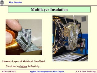
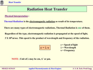
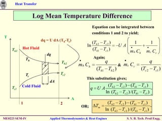
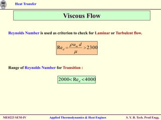
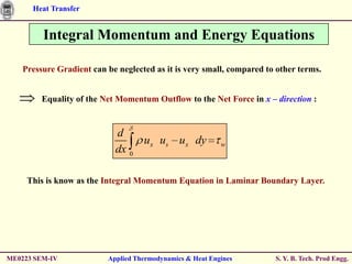
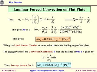
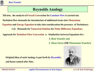
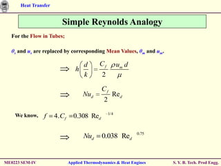
77. Heat Transfer
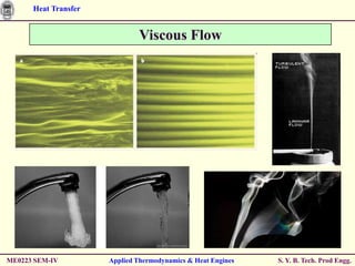
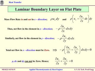
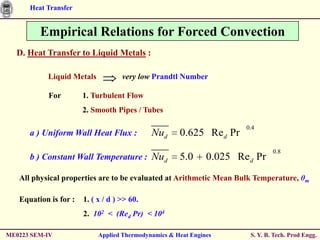
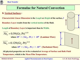
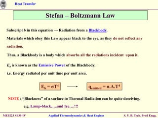
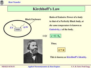
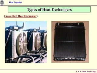
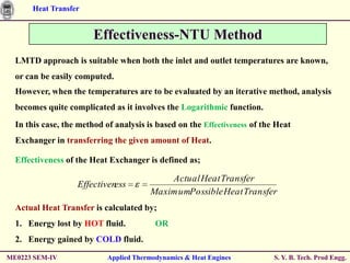
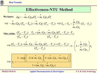
Effectiveness-NTU Method
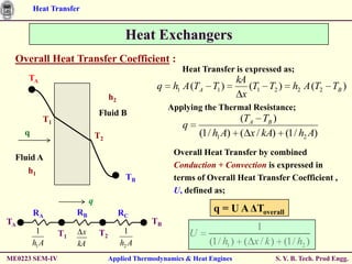
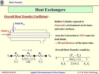
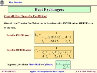
Heat Exchanger Effectiveness Relations :
N = NTU = UA/Cmin C = Cmin/Cmax
Flow Geometry Relation
Double Pipe :
1 exp[ N (1 C )]
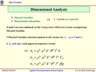
Parallel Flow 1 C
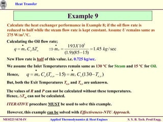
1 exp[ N (1 C )]
Counter Flow
1 C exp[ N (1 C )]
N
Counter Flow, C = 1 N 1
Cross Flow :
exp( NCn) 1 0.22
Both Fluids Mixed 1 exp where n N
Cn 1
1 C 1
Both Fluids Unmixed
1 exp( N ) 1 exp( NC ) N
Cmax mixed, Cmin Unmixed (1/ C){ exp[ C(1 e N )]}
1
Cmax Unmixed, Cmin Mixed 1 exp{ (1 / C )[1 exp( NC )]}
Shell-and-Tube :
1
2 1/ 2 1 exp[ N (1 C 2 )1/ 2 ]
1 Shell-pass; 2/4/6 Tube-pass 2 1 C (1 C ) X
1 exp[ N (1 C 2 )1/ 2 ]
All Exchangers, C = 0 : 1 e N
ME0223 SEM-IV Applied Thermodynamics & Heat Engines S. Y. B. Tech. Prod Engg.

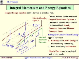
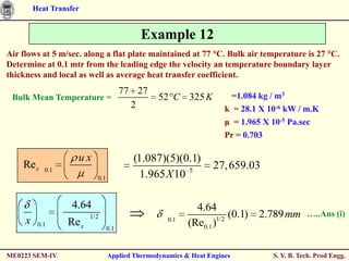
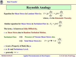
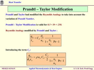
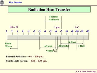
78. Heat Transfer
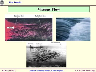
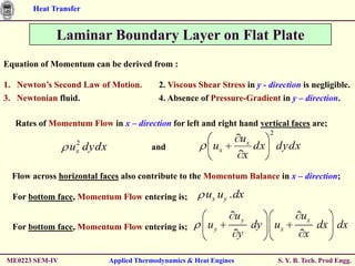
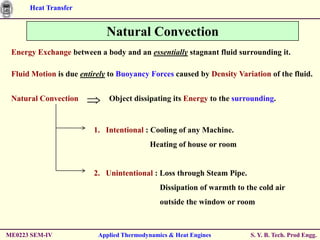
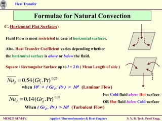
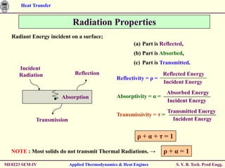
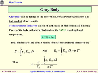
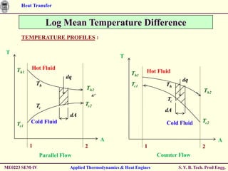
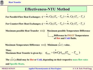
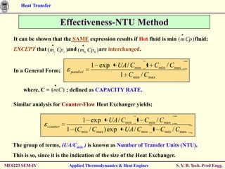
Effectiveness-NTU Method
Heat Exchanger NTU Relations :
N = NTU = UA/Cmin C = Cmin/Cmax ε = Effectiveness
Flow Geometry Relation
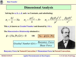
Double Pipe :
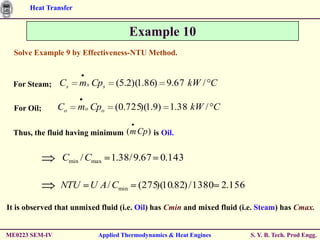
ln[1 (1 C ) ]
Parallel Flow N
1 C
Counter Flow 1 1
N ln
C 1 C 1
Counter Flow, C = 1 N
1
Cross Flow :
1
Cmax mixed, Cmin Unmixed N ln 1 ln (1 C )
C
1
Cmax Unmixed, Cmin Mixed N ln [1 C ln (1 )]
C
Shell-and-Tube :
2 1/ 2 (2 / ) 1 C (1 C 2 )1/ 2
1 Shell-pass; 2/4/6 Tube-pass N (1 C ) X ln
(2 / ) 1 C (1 C 2 )1/ 2
All Exchangers, C = 0 : N ln (1 )
ME0223 SEM-IV Applied Thermodynamics & Heat Engines S. Y. B. Tech. Prod Engg.

79. Heat Transfer
Example 8
A cross-flow heat exchanger is used to heat an oil in the tubes (C=1.9 kJ/kg.ºC) from
15 ºC to 85 ºC. Blowing across the outside of the tubes is steam which enters at 130 ºC
and leaves at 110 ºC with a mass flow rate of 5.2 kg/sec. The overall heat transfer
coefficient is 275 W/m2.ºC and C for steam is 1.86 kJ/kg.ºC. Calculate the surface
area of the heat exchanger.
Total Heat Transfer is calculated from Energy Balance of Steam;
q m s Cs Ts (5.2)(1.86)(130 110) 193 kW T
130 °C Hot Fluid Th
∆Tm is calculated by treating as a dq
Counter-Flow Heat Transfer; 85 °C 110 °C
Tc
(130 85) (110 15)
Tm 66.9 C
(130 85) dA 15 °C
ln
(110 15) Cold Fluid
A
1
ME0223 SEM-IV Applied Thermodynamics & Heat Engines S. Y. B. Tech. Prod Engg.

80. Heat Transfer
Example 8….contd
t1 and t2 represent unmixed fluid (i.e. Oil) and T1 and T2 represent the mixed fluid
(i.e. Steam). Hence;
T1 = 130 ºC; T2 = 110 ºC; t1 = 15 ºC; t2 = 85 ºC
t2 t1 85 15 T1 T2 130 110
P 0.609 And R 0.286
T1 t1 130 15 t2 t1 85 15
From LMTD Correction Chart; F = 0..97
Heat Transfer Area is;
q 193 X 103
A
U F Tm (275)(0.97)(66.9)
10.82 m 2 ….ANS
S. Y. B. Tech. Prod Engg.

81. Heat Transfer
Example 9
Calculate the heat exchanger performance in Example 8; if the oil flow rate is
reduced to half while the steam flow rate is kept constant. Assume U remains same as
275 W/m2.ºC.
Calculating the Oil flow rate;
193X 103
q mo Co To mo 1.45 kg / sec
(1.9)(85 15)
New Flow rate is half of this value. i.e. 0.725 kg/sec.
We assume the Inlet Temperatures remain same as 130 ºC for Steam and 15 ºC for Oil.
Hence, q mo Co (Te,o 15) ms Cs (130 Te,s )
But, both the Exit Temperatures Te,o and Te,s are unknown.
The values of R and P can not be calculated without these temperatures.
Hence, ∆Tm can not be calculated.
ITERATIVE procedure MUST be used to solve this example.
However, this example can be solved with Effectiveness-NTU Approach.
ME0223 SEM-IV Applied Thermodynamics & Heat Engines S. Y. B. Tech. Prod Engg.

82. Heat Transfer
Example 10
Solve Example 9 by Effectiveness-NTU Method.
For Steam; Cs m s Cps (5.2)(1.86) 9.67 kW / C
For Oil; Co mo Cpo (0.725)(1.9) 1.38 kW / C
Thus, the fluid having minimum ( m Cp ) is Oil.
Cmin / Cmax 1.38/ 9.67 0.143
NTU U A / Cmin (275)(10.82) / 1380 2.156
It is observed that unmixed fluid (i.e. Oil) has Cmin and mixed fluid (i.e. Steam) has Cmax.
ME0223 SEM-IV Applied Thermodynamics & Heat Engines S. Y. B. Tech. Prod Engg.

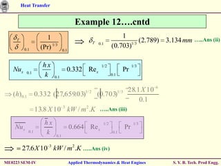
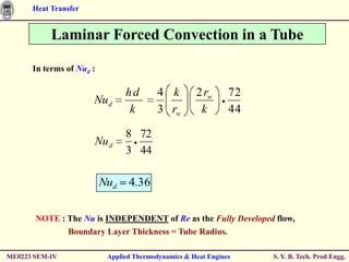
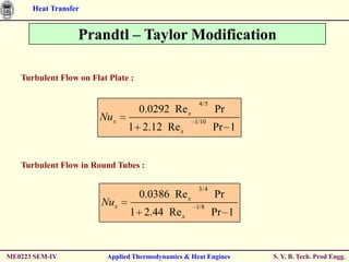
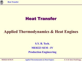
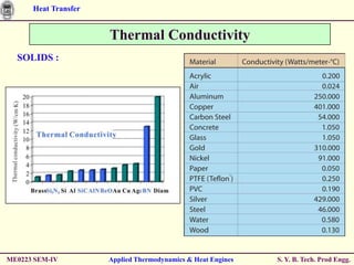
83. Heat Transfer
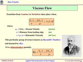
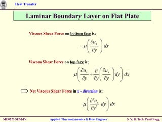
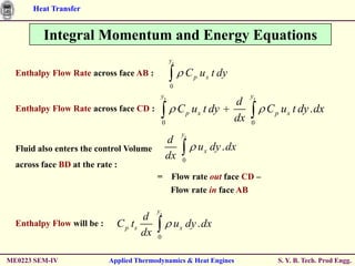
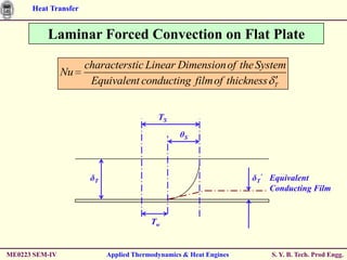
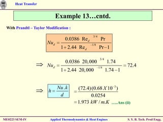
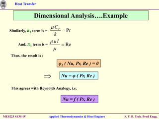
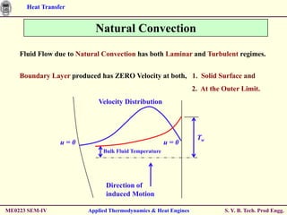
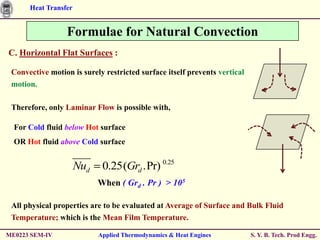
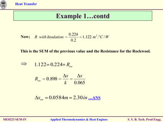
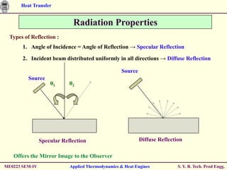
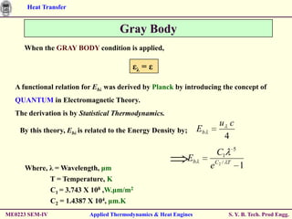
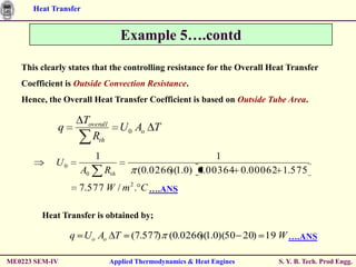
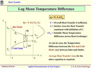
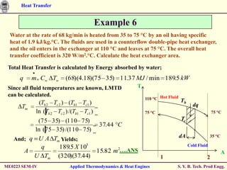
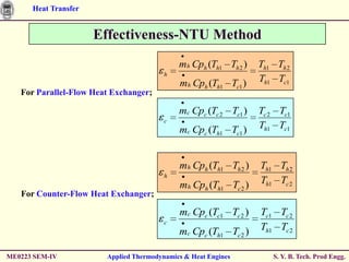
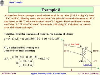
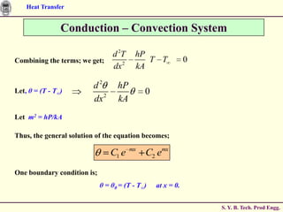
Example 10….contd
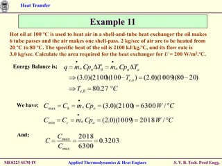
Hence; from the Table; we get;
(1 / C ){1 exp[ C (1 e N )]}
2.156
(1 / 0 / 143) 1 exp[ (0.143)(1 e )] 0.831
Using the Effectiveness, we can calculate the Temperature Difference for Oil as;
To ( Tmax ) (0.831 130 15) 95.5 C
)(
Thus, the Heat Transfer is;
q mo Cpo To (1.38)(95.5) 132 kW
Thus,
Reduction in Oil flow rate by 50 % results in reduction in Heat Transfer by 32 % only.
S. Y. B. Tech. Prod Engg.

84. Heat Transfer
Example 11
Hot oil at 100 ºC is used to heat air in a shell-and-tube heat exchanger the oil makes
6 tube passes and the air makes one shell-pass. 2 kg/sec of air are to be heated from
20 ºC to 80 ºC. The specific heat of the oil is 2100 kJ/kg.ºC, and its flow rate is
3.0 kg/sec. Calculate the area required for the heat exchanger for U = 200 W/m2.ºC.
Energy Balance is; q mo Cpo T0 ma Cpa Ta
(3.0)(2100 100 Te,o ) (2.0)(1009 80 20)
)( )(
Te,0 80.27 C
We have; Cmax Ch mo Cpo (3.0)(2100 6300 W / C
)
Cmin Cc m a Cpa (2.0)(1009) 2018 W / C
And; Cmain 2018
C 0.3203
Cmax 6300
ME0223 SEM-IV Applied Thermodynamics & Heat Engines S. Y. B. Tech. Prod Engg.

85. Heat Transfer
Example 11….contd
Tc (80 20)
Effectiveness is; 0.75
Tmax (100 20)
From the NTU Table;
2 1/ 2 (2 / ) 1 C (1 C 2 )1/ 2
N (1 C ) X ln
(2 / ) 1 C (1 C 2 )1/ 2
2 1/ 2 (2 / 0.75) 1 0.3203 (1 0.32032 )1/ 2
(1 0.3203 ) X ln
(2 / 0.75) 1 0.3203 (1 0.32032 )1/ 2
1.99
UA
NTU
Thus;
Cmin
Cmin (2018 ) 2
A NTU (2.1949) 22.146 m….ANS
U (200)
ME0223 SEM-IV Applied Thermodynamics & Heat Engines S. Y. B. Tech. Prod Engg.

86. Heat Transfer
Convection Heat Transfer
T∞ Consider a heated plate shown in Fig.
u∞
Temperature of the plate is Tw and that of
surrounding is T∞
u
q Velocity profile is as shown in Fig.
Tw
Velocity reduces to Zero at the plate surface as
a result of Viscous Action.
Since no velocity at the plate surface, Heat is transferred by Conduction only.
Then , WHY Convection ?
ANS : Temperature Gradient depends on the rate at which fluid carries away the Heat.
Overall Effect of Convection is given by Newton’s Law of Cooling.
q = h A ΔT = h A (Tw - T∞)
h is known as the CONVECTIVE HEAT TRANSFER COEFFICIENT. (W/m2.K)
S. Y. B. Tech. Prod Engg.

87. Heat Transfer
Convection Heat Transfer
T∞ Convective Heat Transfer has dependence
u∞
on Viscosity as well as Thermal properties of
u the fluid.
q
Tw 1) Thermal Conductivity, k
2) Specific Heat, Cp
3) Density, ρ
Heated plate exposed to room air; without any external source of motion of fluid, the
movement of air will be due to the Density Gradient.
This is called Natural or Free Convection.
Heated plate exposed to air blown by a fan; i.e. with an external source of motion of fluid.
This is called Forced Convection.
S. Y. B. Tech. Prod Engg.

88. Heat Transfer
Convection Energy Balance on Flow Channel
The same analogy can be used for evaluating the
Heat Loss / Gain resulting from a fluid flowing
Te Ti inside a channel or tube, as shown in Fig.
Heated wall at temperature Tw loses heat to the
m
cooler fluid through the channel (i.e. pipe).
Temperature rise from inlet (Ti) to exit (Te).
q
q m Cp (Te Ti ) h A (Tw,avg T fluid,avg )
Te, Ti and Tfluid are known as Bulk or Energy Average
Temperatures.
S. Y. B. Tech. Prod Engg.

89. Heat Transfer
Convection Boundary Condition
We know that;
qconv h A (Tw T )
With Electrical Analogy, as in case of Conduction;
(Tw T )
qconv
1
hA
The term
1 is known as Convective Resistance;
hA
ME0223 SEM-IV Applied Thermodynamics & Heat Engines S. Y. B. Tech. Prod Engg.

90. Heat Transfer
Conduction – Convection System
Heat conducted through a body, frequently needs to be removed by Convection process.
e.g. Furnace walls, Motorcycle Engine, etc.
Finned Tube arrangement is the most common for such Heat Exchange applications.
Consider a One – Dimensional fin.
dqconv =h P dx (T-T∞)
t Surrounding fluid at T∞.
Base of fin at T0.
A
qx Qx+x Energy Balance of element of fin with thickness dx ;
dx
Energy in left face = Energy out right face +
L
Energy lost by Convection
Base
S. Y. B. Tech. Prod Engg.

91. Heat Transfer
Conduction – Convection System
Convection Heat Transfer; qconv h A (Tw T )
Where, Area of fin is surface area for Convection.
Let the C/s. area be A and perimeter be P.
dT
Energy in left face; qx kA
dx
dT dT d 2T
Energy out right face; qx dx kA kA 2
dx
dx x dx dx dx
Energy lost by Convection; qconv h P dx (T T )
NOTE : Differential area of the fin is the product of Perimeter and the differential
length dx.
ME0223 SEM-IV Applied Thermodynamics & Heat Engines S. Y. B. Tech. Prod Engg.

92. Heat Transfer
Conduction – Convection System
d 2T hP
Combining the terms; we get; T T 0
dx 2 kA
d2 hP
Let, θ = (T - T∞) 0
dx 2 kA
Let m2 = hP/kA
Thus, the general solution of the equation becomes;
mx
C1 e C2 emx
One boundary condition is;
θ = θ0 = (T - T∞) at x = 0.
S. Y. B. Tech. Prod Engg.

93. Heat Transfer
Conduction – Convection System
Other boundary conditions are;
CASE 1 : Fin is very long.
Temperature at the fin end is that of surrounding.
CASE 2 : Fin has finite length.
Temperature loss due to Convection.
CASE 3 : Fin end is insulated.
dT/dx = 0 at x = L.
For CASE 1, Boundary Conditions are : θ = θ0 = (T - T∞) at x = 0.
θ=0 at x = ∞.
T T mx
And, the solution becomes; e
0 T0 T
ME0223 SEM-IV Applied Thermodynamics & Heat Engines S. Y. B. Tech. Prod Engg.

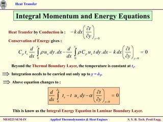
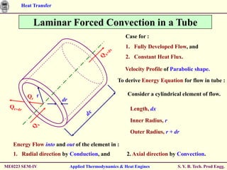
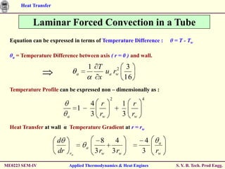
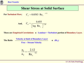
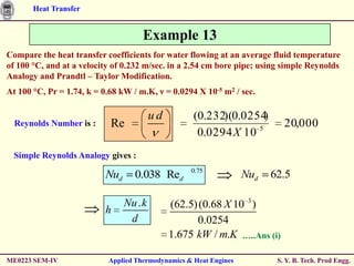
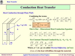
94. Heat Transfer
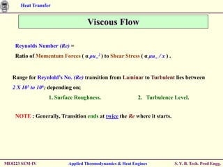
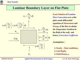
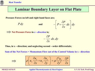
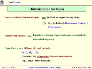
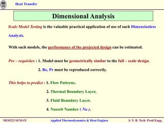
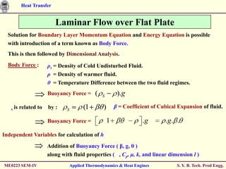
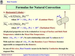
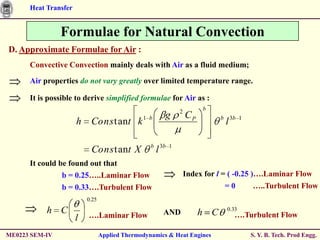
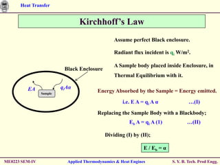
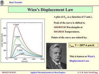
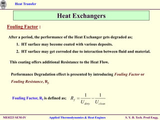
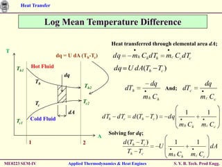
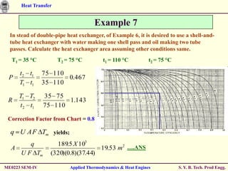
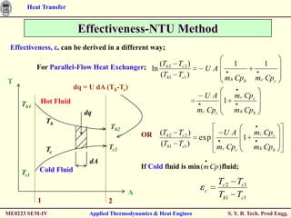
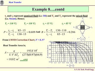
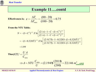
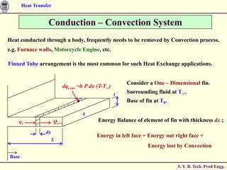
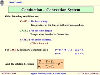
Conduction – Convection System
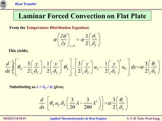
For CASE 3, Boundary Conditions are : θ = θ0 = (T - T∞) at x = 0.
dθ/dx = 0 at x = L.
This yields;
0 C1 C2
mL
0 m ( C1 e C2 e mL )
e mx emx cosh[m ( L x)]
Solving for C1 and C2, we get;
0 1 e 2mL 1 e2mL cosh (mL)
where, the hyperbolic functions are defined as;
ex e x
ex e x
ex e x
sinh x cosh x tanh x
2 2 ex e x
ME0223 SEM-IV Applied Thermodynamics & Heat Engines S. Y. B. Tech. Prod Engg.

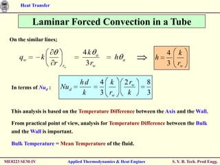
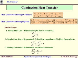
95. Heat Transfer
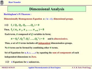
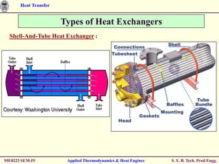
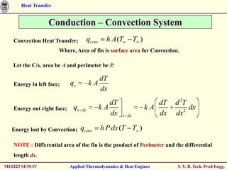
Conduction – Convection System
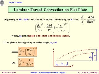
Solution for CASE 2 is;
T T cosh[m ( L x)] (h / mk )sinh[m ( L x)]
T0 T cosh (mL) (h / mk )sinh (mL)
All the Heat loss by the fin MUST be conducted to the base of fin at x = 0.
dT
Thus, the Heat loss is; qx dx kA
dx x 0
Alternate method of integrating Convection Heat Loss;
L L
q h P (T T ) dx h P dx
0 0
ME0223 SEM-IV Applied Thermodynamics & Heat Engines S. Y. B. Tech. Prod Engg.

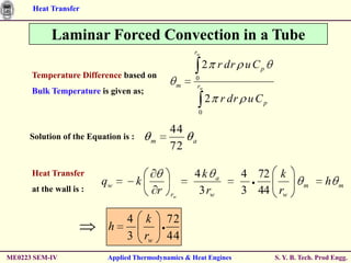
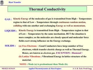
96. Heat Transfer
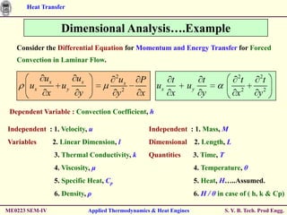
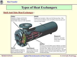
Conduction – Convection System
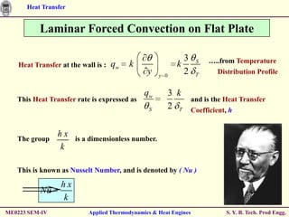
Application of Conduction equation is easier than that for Convection.
m(0)
For CASE 1 : q k A[ m 0e ] h Pk A 0
1 1
q kA 0m
1 e 2 mL 1 e 2 mL
For CASE 3 :
hPk A 0 tanh (mL)
sinh (mL) (h / mk ) cosh (mL)
For CASE 2 : q hPk A 0
cosh (mL) (h / mk )sinh (mL)
ME0223 SEM-IV Applied Thermodynamics & Heat Engines S. Y. B. Tech. Prod Engg.

97. Heat Transfer
Viscous Flow
A) Flow over a Flat Plate :
Laminar Transition Turbulent y
du
dy
u∞ x
u
u∞ Laminar
Sublayer
u
At the leading edge of the plate, a region develops, where the influence of Viscous Forces
is felt.
These viscous forces are described in terms of Shear Stress, η, between the fluid layers.
ME0223 SEM-IV Applied Thermodynamics & Heat Engines S. Y. B. Tech. Prod Engg.

98. Heat Transfer
Viscous Flow
Shear Stress is proportional to normal velocity gradient.
du
dy
The constant of proportionality, μ, is known as dynamic viscosity. (N-sec/m2)
Region of flow, developed from the leading edge, in which the effects of Viscosity are
observed, is known as Boundary Layer.
The point for end of Boundary Layer is chosen as the y co-ordinate where the velocity
becomes 99 % of the free – stream value.
Initial development of Boundary Layer is Laminar.
After some critical distance from leading edge, small disturbances in flow get amplified.
This transition is continued till the flow becomes Turbulent.
S. Y. B. Tech. Prod Engg.

99. Heat Transfer
Viscous Flow
Laminar Transition Turbulent
Turbulent Transition Laminar
Development of Flow Regimes
ME0223 SEM-IV Applied Thermodynamics & Heat Engines S. Y. B. Tech. Prod Engg.

100. Heat Transfer
Viscous Flow
ME0223 SEM-IV Applied Thermodynamics & Heat Engines S. Y. B. Tech. Prod Engg.

101. Heat Transfer
Viscous Flow
ME0223 SEM-IV Applied Thermodynamics & Heat Engines S. Y. B. Tech. Prod Engg.

102. Heat Transfer
Viscous Flow
ME0223 SEM-IV Applied Thermodynamics & Heat Engines S. Y. B. Tech. Prod Engg.

103. Heat Transfer
Viscous Flow
Transition from Laminar to Turbulent takes place when;
u x u x
5 X 105
where,
u∞ = Free – Stream Velocity (m/sec)
x = Distance from leading edge (m)
ν = μ / ρ = Kinematic Viscosity (m2/sec)
This particular group of terms is known as Reynold’s Number;
and denoted by (Re).
It is a dimensionless quantity.
u x u x
Re
ME0223 SEM-IV Applied Thermodynamics & Heat Engines S. Y. B. Tech. Prod Engg.

104. Heat Transfer
Viscous Flow
Reynolds Number (Re) =
Ratio of Momentum Forces ( α ρu∞2 ) to Shear Stress ( α μu∞ / x ) .
Range for Reynlold’s No. (Re) transition from Laminar to Turbulent lies between
2 X 105 to 106; depending on;
1. Surface Roughness. 2. Turbulence Level.
NOTE : Generally, Transition ends at twice the Re where it starts.
ME0223 SEM-IV Applied Thermodynamics & Heat Engines S. Y. B. Tech. Prod Engg.

105. Heat Transfer
Viscous Flow
Laminar Transition Turbulent y
du
dy
u∞ x
u
u∞ Laminar
Sublayer
u
Laminar profile is approximately Parabolic.
Turbulent profile has a initial part, close to plate, is very nearly Linear.
This is due to the Laminar Sublayer that adheres to the surface.
Portion outside this Sublayer is relatively Flat.
ME0223 SEM-IV Applied Thermodynamics & Heat Engines S. Y. B. Tech. Prod Engg.

106. Heat Transfer
Viscous Flow
Physical mechanism of Viscosity Momentum Transfer
Laminar flow Molecules move from one lamina to another,
carrying Momentum α Velocity
Net Momentum Transfer from High Velocity region to Low Velocity Region.
Force in direction of flow, i.e. Viscous shear Stress, η
Rate of Momentum Transfer α Rate of movement of molecules α T
Turbulent flow has no distinct fluid layers.
Macroscopic chunks of fluid, transporting Energy and Momentum,
in stead of microscopic molecular motion.
Larger Viscous shear Stress, η
ME0223 SEM-IV Applied Thermodynamics & Heat Engines S. Y. B. Tech. Prod Engg.

107. Heat Transfer
Viscous Flow
B) Flow through a Pipe :
Boundary Layer
Uniform
Inlet
Flow
Starting Length
Fully Developed Flow
Laminar
Sublayer
(A) Laminar Flow
Turbulent Core (B) Turbulent flow
ME0223 SEM-IV Applied Thermodynamics & Heat Engines S. Y. B. Tech. Prod Engg.

108. Heat Transfer
Viscous Flow
Boundary Layer develops at the entrance of the pipe.
Eventually, the Boundary Layer fills entire tube. The flow is said to be fully developed.
For Laminar flow, Parabolic velocity profile is developed.
For Turbulent flow, a somewhat blunter profile is observed.
Velocity profiles can be mathematically expressed as :
u y y
For Laminar flow : 2
um r r
1
For Turbulent flow : u y 7
um r
ME0223 SEM-IV Applied Thermodynamics & Heat Engines S. Y. B. Tech. Prod Engg.

109. Heat Transfer
Viscous Flow
Reynolds Number is used as criterion to check for Laminar or Turbulent flow.
um d
Re d 2300
Range of Reynolds Number for Transition :
2000 Red 4000
ME0223 SEM-IV Applied Thermodynamics & Heat Engines S. Y. B. Tech. Prod Engg.

110. Heat Transfer
Viscous Flow
Continuity Equation for One-dimensional flow in a tube ;
m um A
where, m = Mass Flow Rate (kg / sec);
um = Mean Velocity (m / sec);
A = Cross-Sectional Area (m2).
Mean Velocity, G can be defined as;
m
G um
A
Reynolds Number, Re can also be written as;
Gd
Re d
ME0223 SEM-IV Applied Thermodynamics & Heat Engines S. Y. B. Tech. Prod Engg.

111. Heat Transfer
Inviscid Flow
No Real fluid is inviscid.
Practically, we can assume the flow to be inviscid for certain conditions.
Flow at a sufficiently large distance from the flat plate, can be assumed to be inviscid.
Velocity Gradients, normal to the direction of flow are very small.
Viscous – Shear Forces are also very small.
Balance of Forces on an element of Incompressible fluid
= Change in Momentum of fluid element; yields Bernoulli’s Equation as;
P 1V2 where, ρ = Fluid Density, (kg/m3)
Const.
2 g P = Pressure at particular point in flow, (Pa)
V = Velocity of flow at that point, (m/sec)
ME0223 SEM-IV Applied Thermodynamics & Heat Engines S. Y. B. Tech. Prod Engg.

112. Heat Transfer
Inviscid Flow
Bernoulli’s Equation is considered as Energy Equation due to ;
1. The term ( V2 / 2g ) ≡ Kinetic Energy.
2. The term ( P / γ ) ≡ Potential Energy.
For a Compressible fluid, Energy Equation should take into account :
1. Changes in Internal Energy, h
2. Corresponding changes in Temperatures, T.
ME0223 SEM-IV Applied Thermodynamics & Heat Engines S. Y. B. Tech. Prod Engg.

113. Heat Transfer
Inviscid Flow
One – Dimensional Steady – Flow Energy Equation :
2 2
V1 V2
h1 Q h2 W
2g 2g
h is the Enthalpy of the state and is defined as;
h u Pv
where, u = Internal Energy, (Joule)
Q = Heat added to Control Volume, (Joule)
W = Net Work done in the Process, (Joule)
v = Specific Volume of fluid, (m3/kg)
ME0223 SEM-IV Applied Thermodynamics & Heat Engines S. Y. B. Tech. Prod Engg.

114. Heat Transfer
Compressible Fluid Flow
Equations of State of the fluid ;
P=ρRT Δu = Cv ΔT Δh = Cp ΔT
Gas Constant for a gas is given as;
R=R /M
where, M = Molecular Weight of the gas.
R = Universal Gas Constant = 8314.5 J/kg.mol.K
For Air, the Ideal Gas Properties are :
Rair = 287 J/kg.K Cv, air = 0.718 kJ/kg.K
Cp, air = 1.005 kJ/kg.K γair = Cp / Cv = 1.4
ME0223 SEM-IV Applied Thermodynamics & Heat Engines S. Y. B. Tech. Prod Engg.

115. Heat Transfer
Thermal Boundary Layer
On similar lines of Velocity Boundary Layers, there exist Thermal Boundary Layers also.
Laminar Transition Turbulent
T∞
T
T∞
T
Flow regions where the fluid temperature changes from the free – stream value to the
value at the surface.
Thermal Boundary Layer thickness δT = Distance from surface in y – direction
where, ( T – Tw ) / ( T∞ - Tw ) = 0.99 or 99 %
ME0223 SEM-IV Applied Thermodynamics & Heat Engines S. Y. B. Tech. Prod Engg.

116. Heat Transfer
Laminar Boundary Layer on Flat Plate
uy Exact Solution of Laminar
uy dy
y Flow Convection over a flat
plate needs differential
ux 2
ux equations of Momentum and
dx dx 2
dy Energy of the flow to obtain
y y
ux the Temperature Gradient in
ux dx
ux x the fluid at the wall, and
P hence, Convection Coefficient.
P dx dy
P dy x
Assumptions :
ux
dx
y 1. Steady – State conditions,
2. Unit Depth,
uy 3. Fluid Densiy, ρ
ME0223 SEM-IV Applied Thermodynamics & Heat Engines S. Y. B. Tech. Prod Engg.

117. Heat Transfer
Laminar Boundary Layer on Flat Plate
ux
Mass Flow Rate in and out in x – direction; u x dy and ux dx dy
x
ux
Thus, net flow in the element in x – direction; dx dy
x
uy
Similarly, net flow in the element in y – direction; dy dx
y
ux uy
Total net flow in x – direction must be Zero. dx dy 0
x y
ux uy
ρ, dx and dy can not be Zero. Hence; 0
x y
ME0223 SEM-IV Applied Thermodynamics & Heat Engines S. Y. B. Tech. Prod Engg.

118. Heat Transfer
Laminar Boundary Layer on Flat Plate
Equation of Momentum can be derived from :
1. Newton’s Second Law of Motion. 2. Viscous Shear Stress in y - direction is negligible.
3. Newtonian fluid. 4. Absence of Pressure-Gradient in y – direction.
Rates of Momentum Flow in x – direction for left and right hand vertical faces are;
2
2 ux
ux dy dx and ux dx dy dx
x
Flow across horizontal faces also contribute to the Momentum Balance in x – direction;
For bottom face, Momentum Flow entering is; ux u y . dx
uy ux
For bottom face, Momentum Flow entering is; uy dy ux dx dx
y x
ME0223 SEM-IV Applied Thermodynamics & Heat Engines S. Y. B. Tech. Prod Engg.

119. Heat Transfer
Laminar Boundary Layer on Flat Plate
Viscous Shear Force on bottom face is;
ux
dx
y
Viscous Shear Force on top face is;
ux ux
dy dx
y y y
Net Viscous Shear Force in x - direction is;
2
ux
2
dy dx
y
ME0223 SEM-IV Applied Thermodynamics & Heat Engines S. Y. B. Tech. Prod Engg.

120. Heat Transfer
Laminar Boundary Layer on Flat Plate
Pressure Forces on left and right hand faces are;
P
P dy and P dx dy
x
Net Pressure Force in x - direction is;
P
dx . dy
x
Thus, in x – direction; and neglecting second – order differentials;
Sum of the Net Forces = Momentum Flow out of the Control Volume in x - direction
2
ux ux ux P
ux uy
x y y2 x
ME0223 SEM-IV Applied Thermodynamics & Heat Engines S. Y. B. Tech. Prod Engg.

121. Heat Transfer
Laminar Boundary Layer on Flat Plate
On the similar lines to that with Momentum Equation; the Energy Equation can also be
derived as;
2
t t uy t
k dx dy Cp uy dy t dy dx
y y2 y y
ux t
Cp ux t dy C p ux dx t dx dy
x x
2
t t t
k dy k dy 2
dx
x x x
Energy Balance =
t Rate of Net Conduction in
k dx Cp uy t dx
y + Rate of Net Convection in
=0
ME0223 SEM-IV Applied Thermodynamics & Heat Engines S. Y. B. Tech. Prod Engg.

122. Heat Transfer
Laminar Boundary Layer on Flat Plate
i.e. 2 2
t t
k dx dy
x2 y2
t ux ux t
Cp u x t dx dy
x x x x
t uy uy t
Cp u y t dx dy 0
y y y y
2 2
t t t t
OR ux uy
x y x2 y2
ME0223 SEM-IV Applied Thermodynamics & Heat Engines S. Y. B. Tech. Prod Engg.

123. Heat Transfer
Laminar Boundary Layer on Flat Plate
2
t
Conduction in x – direction 2
is very small and can be neglected.
x
2 2
t t t t
ux uy
x y x2 y2
P
Similarly, Pressure Gradient in x – direction is also small and can be neglected.
x
2
ux ux ux P
ux uy
x y y2 x
ME0223 SEM-IV Applied Thermodynamics & Heat Engines S. Y. B. Tech. Prod Engg.

124. Heat Transfer
Laminar Boundary Layer on Flat Plate
Similarities between Momentum Equation and energy Equation ;
ux ux 2
ux 2
ux ν is the Kinematic Viscosity
ux uy or Momentum Diffusivity
x y y2 y2 =μ/ρ
2
t t t
ux uy
x y y2
k Cp Diffusion of Momentum
Pr /
Cp k Diffusion of Energy
This dimensionless Number that relates Fluid Boundary Layer and
Thermal Boundary Layer is known as Prandtl No. and denoted by ( Pr ).
ME0223 SEM-IV Applied Thermodynamics & Heat Engines S. Y. B. Tech. Prod Engg.

125. Heat Transfer
Laminar Boundary Layer on Flat Plate
Pr < 1 Pr = 1 Pr > 1
u
δ = δT
T∞ δ δT δT δ
Prandtl No. can vary from 4 X 10-3 – 0.2 and 1.0 - 4 X 104
Liquid Metals Viscous Oils
Gases have generally Pr = 0.7
ME0223 SEM-IV Applied Thermodynamics & Heat Engines S. Y. B. Tech. Prod Engg.

126. Heat Transfer
Integral Momentum and Energy Equations
Consider a Control Volume that extends
from wall to just beyond the limit of
D
Boundary Layer in y – direction.
B Thickness dx in x – direction.
C
y=δ
Unit depth in z – direction.
A
y
Equation to relate Net Momentum Outflow
to Net Force acting in x – direction.
ME0223 SEM-IV Applied Thermodynamics & Heat Engines S. Y. B. Tech. Prod Engg.

127. Heat Transfer
Integral Momentum and Energy Equations
2
Momentum Flow across face AB : u x dy
0
2 d 2
Momentum Flow across face CD : ux dy ux dy . dx
0
dx 0
d
Fluid also enters the control Volume ux dy . dx
dx 0
across face BD with rate of :
= Fluid leaving across face CD –
Fluid entering across face AB
Fluid entering across face BD has Velocity us in x – direction.
d
Momentum Flow into Control Volume in x – direction : us ux dy . dx
dx 0
ME0223 SEM-IV Applied Thermodynamics & Heat Engines S. Y. B. Tech. Prod Engg.

128. Heat Transfer
Integral Momentum and Energy Equations
Net Momentum Outflow in x – direction :
d d
ux dy . dx us ux dy . dx
dx 0 dx 0
Pressure Force will act on face AB and CD.
Shear Force will act on face AC.
No Shear Force will act on face BD since it is at limit of Boundary Layer.
ux
0
y
Net Force acting on Control Volume in x – direction :
Px Px
Px Px dx w dx dx w dx
x x
ME0223 SEM-IV Applied Thermodynamics & Heat Engines S. Y. B. Tech. Prod Engg.

129. Heat Transfer
Integral Momentum and Energy Equations
Pressure Gradient can be neglected as it is very small, compared to other terms.
Equality of the Net Momentum Outflow to the Net Force in x – direction :
d
ux us ux dy w
dx 0
This is know as the Integral Momentum Equation in Laminar Boundary Layer.
ME0223 SEM-IV Applied Thermodynamics & Heat Engines S. Y. B. Tech. Prod Engg.

130. Heat Transfer
Integral Momentum and Energy Equations
Integral Energy Equation can be derived in a similar way.
Control Volume similar to that of
Velocity Boundary
Integral Momentum Equation is
Layer, δ
considered, but extending beyond
D the limits of both Velocity
Boundary Layer and Thermal
Boundary Layer.
B Principle of Conservation of Energy
C
Thermal applied involves :
Boundary 1. Enthalpy and Kinetic Energy of
Layer, δT
A Fluid entering and leaving.
y 2. Heat Transfer by Conduction.
Kinetic Energy can be neglected
as it is very small.
ME0223 SEM-IV Applied Thermodynamics & Heat Engines S. Y. B. Tech. Prod Engg.

131. Heat Transfer
Integral Momentum and Energy Equations
ys
Enthalpy Flow Rate across face AB : C p u x t dy
0
ys ys
d
Enthalpy Flow Rate across face CD : C p ux t dy C p u x t dy . dx
0
dx 0
ys
d
Fluid also enters the control Volume u x dy . dx
dx 0
across face BD at the rate :
= Flow rate out face CD –
Flow rate in face AB
ys
d
Enthalpy Flow will be : C p ts u x dy . dx
dx 0
ME0223 SEM-IV Applied Thermodynamics & Heat Engines S. Y. B. Tech. Prod Engg.

132. Heat Transfer
Integral Momentum and Energy Equations
t
Heat Transfer by Conduction is : k dx
y y 0
Conservation of Energy gives :
ys ys
d d t
C p ts u x dy . dx C p u x t dy . dx k dx 0
dx 0
dx 0
y y 0
Beyond the Thermal Boundary Layer, the temperature is constant at ts.
Integration needs to be carried out only up to y = δT.
Above equation changes to :
T
d t
ts t u x dy 0
dx 0
y y 0
This is know as the Integral Energy Equation in Laminar Boundary Layer.
ME0223 SEM-IV Applied Thermodynamics & Heat Engines S. Y. B. Tech. Prod Engg.

133. Heat Transfer
Laminar Forced Convection on Flat Plate
Integral Momentum Equation and Integral Energy Equation are applied to solve the
equation for Laminar Forced Convection.
Analysis assumes uniform Viscosity with Temperature.
STEP 1 :
Apply Integral Momentum Equation to derive for Velocity Boundary Layer Thickness.
Velocity profile assumed to be : ux = a + by + cy2 + dy3
Constants a, b, c and d are found by applying known Boundary Conditions :
ux = 0 at y = 0. a = 0. ux
0 at y = δ
y 2
ux = us at y = δ. ux
ux and uy = 0 0 at y = 0
y2
3 us - 1 us
This yields; b= c=0 d=
2 δ 2 δ3
ME0223 SEM-IV Applied Thermodynamics & Heat Engines S. Y. B. Tech. Prod Engg.

134. Heat Transfer
Laminar Forced Convection on Flat Plate
3
ux 3 y 1 y
This yields;
us 2 2
STEP 2 :
Apply Integral Momentum Equation,
d
ux us ux dy w
dx 0
3 3
d 3 y 1 y 3 y 1 y
us2 . 1 dy
dx 0
2 2 2 2
du x
dy y 0
ME0223 SEM-IV Applied Thermodynamics & Heat Engines S. Y. B. Tech. Prod Engg.

135. Heat Transfer
Laminar Forced Convection on Flat Plate
3 us
Wall Shear Stress is found by considering Velocity Gradient at y = 0 and is =
2 δ
d 2 39 3 us 2 3 280 us
u
s u d
s dx
dx 280 2 2 39
2
140 140 x
d dx Integration yields; C
13 us 2 13 us
δ = 0 at x = 0. C=0
2 280 x
13 us
OR
4.64
x (Re)1/ 2
ME0223 SEM-IV Applied Thermodynamics & Heat Engines S. Y. B. Tech. Prod Engg.

136. Heat Transfer
Laminar Forced Convection on Flat Plate
Temperature Distribution in the Thermal Boundary Layer can be found out in similar
manner.
STEP 1 :
Temperature profile assumed to be : θx = ( t – tw ) = dy + ey2 + fy3
Applying the known Boundary Conditions and solving for the constants d, e and f ;
3
3 y 1 y
s 2 T 2 T
STEP 2 :
Apply Integral Energy Equation,
T
d
s u x dy 0
dx 0
y y 0
ME0223 SEM-IV Applied Thermodynamics & Heat Engines S. Y. B. Tech. Prod Engg.

137. Heat Transfer
Laminar Forced Convection on Flat Plate
From the Temperature Distribution Equation;
3 s
y y 0
2 T
This yields;
3 3
T
d 3 y 1 y 3 y 1 y 3 s
S S . uS uS dy
dx 0
2 T 2 T 2 T 2 T 2 T
Substituting as λ = δT / δ; gives;
d 3 3 3 3 s
S uS T
dx 20 280 2 T
ME0223 SEM-IV Applied Thermodynamics & Heat Engines S. Y. B. Tech. Prod Engg.

138. Heat Transfer
Laminar Forced Convection on Flat Plate
4.64
Neglecting as 3λ3 / 280 as very small term; and substituting for δ from;
x (Re)1/2
3 3/4
T 0.93 xh
1
Pr x
where, xh is the length of the start of the heated section.
If the plate is heating along its entire length, xh = 0
1/3 y
T 0.93
Pr δ
δT
T 1
OR xh
(Pr)1/3 x
ME0223 SEM-IV Applied Thermodynamics & Heat Engines S. Y. B. Tech. Prod Engg.

139. Heat Transfer
Laminar Forced Convection on Flat Plate
3 S …..from Temperature
Heat Transfer at the wall is : qw k k
y y 0
2 T Distribution Profile
qw 3 k
This Heat Transfer rate is expressed as and is the Heat Transfer
S 2 T Coefficient, h
The group
hx is a dimensionless number.
k
This is known as Nusselt Number, and is denoted by ( Nu )
hx
Nu
k
ME0223 SEM-IV Applied Thermodynamics & Heat Engines S. Y. B. Tech. Prod Engg.

140. Heat Transfer
Laminar Forced Convection on Flat Plate
characterstic Linear Dimension of the System
Nu
Equivalent conducting film of thickness T
TS
θS
δT δT’ Equivalent
Conducting Film
Tw
ME0223 SEM-IV Applied Thermodynamics & Heat Engines S. Y. B. Tech. Prod Engg.

141. Heat Transfer
Laminar Forced Convection on Flat Plate
k k hx x
Thus, qw h S . S h Nu
T T k T
qw x 3 x 3 x (Re)1/2 (Pr)1/3
This gives Nu as ; Nux
S k 2 T 2(0.93)1/3 (4.64) x
This gives ; Nux 0.332(Rex ) 1/ 2 (Pr)1/ 3
This gives Local Nusselt Number at some point x from the leading edge of the plate.
The average value of the Convection Coefficient, h over the distance of 0 to x is given by;
x
1
h h dx
x0
Thus, Average Nusselt No. is; Nux 0.664(Rex ) 1/ 2 (Pr)1/ 3
ME0223 SEM-IV Applied Thermodynamics & Heat Engines S. Y. B. Tech. Prod Engg.

142. Heat Transfer
Example 12
Air flows at 5 m/sec. along a flat plate maintained at 77 °C. Bulk air temperature is 27 °C.
Determine at 0.1 mtr from the leading edge the velocity an temperature boundary layer
thickness and local as well as average heat transfer coefficient.
77 27 =1.084 kg / m3
Bulk Mean Temperature = 52 C 325 K
2 k = 28.1 X 10-6 kW / m.K
μ = 1.965 X 10-5 Pa.sec
Pr = 0.703
ux (1.087)(5)(0.1)
Re x 0.1
27, 659.03
0.1 1.965 X 10 5
4.64 4.64
1/2 (0.1) 2.789 mm …..Ans (i)
x 0.1 Re x 0.1
(Re0.1 )1/2
0.1
ME0223 SEM-IV Applied Thermodynamics & Heat Engines S. Y. B. Tech. Prod Engg.

143. Heat Transfer
Example 12….cntd
1 1
T
T (2.789) 3.134 mm …..Ans (ii)
0.1 1/3
0.1 (Pr) 1/3 (0.703)
0.1
hx 1/2 1/3
Nux 0.1
0.332 Re x Pr
k 0.1
0.1
1/ 2 1/ 3 28.1 X 10 6
(h) 0.1 0.332 (27,659.03) (0.703)
0.1
13.8 X 10 3 kW / m 2 .K …..Ans (iii)
hx 1/2 1/3
Nu x 0.664 Re x Pr
0.1 k 0.1
0.1
27.6 X 10 3 kW / m2 .K …..Ans (iv)
ME0223 SEM-IV Applied Thermodynamics & Heat Engines S. Y. B. Tech. Prod Engg.

144. Heat Transfer
Laminar Forced Convection in a Tube
Case for :
1. Fully Developed Flow, and
2. Constant Heat Flux.
Velocity Profile of Parabolic shape.
To derive Energy Equation for flow in tube :
Consider a cylindrical element of flow.
Length, dx
Inner Radius, r
Outer Radius, r + dr
Energy Flow into and out of the element in :
1. Radial direction by Conduction, and 2. Axial direction by Convection.
ME0223 SEM-IV Applied Thermodynamics & Heat Engines S. Y. B. Tech. Prod Engg.

145. Heat Transfer
Laminar Forced Convection in a Tube
T
Conduction into the element : Qr k 2 r dx
r
Qr T
With change of radius dr, Conduction rate : dr k 2 dx r dr
r r r
This change in Conduction rate = Difference between Convection rates into and
out of the element in Axial Direction.
Temperature changes in Axial Direction.
Rate of Convection into the element : 2 r dr u C p T
T
Rate of Convection out of the element : 2 r dr u C p T dx
x
T
Hence, the difference is : 2 r dr u Cp dx
x
ME0223 SEM-IV Applied Thermodynamics & Heat Engines S. Y. B. Tech. Prod Engg.

146. Heat Transfer
Laminar Forced Convection in a Tube
Summation of total Forces is zero.
1 T Cp T
r
ur r r k x
This is the ENERGY EQUATION FOR LAMINAR FLOW IN TUBES.
Assumptions :
1. Constant Heat Flow, qw,
2. Constant Fluid properties,
Temperature of the fluid (at any radius) must T
Cons tan t
increase linearly in the direction of flow. x
ME0223 SEM-IV Applied Thermodynamics & Heat Engines S. Y. B. Tech. Prod Engg.

147. Heat Transfer
Laminar Forced Convection in a Tube
Boundary Conditions :
1.
T 2. T Tw at r rw
0 at r 0
r
T Heat Flux is related to Temperature Gradient.
3. qw k at r rw
r rw
T
Cons tan t equation reduces to Total Differential Equation.
x
Velocity, u α Velocity at the Axis of tube, ua and Radius, r.
2
u r
1 ….assuming Parabolic Distribution.
ua rw ….rw = wall radius.
ME0223 SEM-IV Applied Thermodynamics & Heat Engines S. Y. B. Tech. Prod Engg.

148. Heat Transfer
Laminar Forced Convection in a Tube
2
Substituting this value in the T 1 T r
r ua 1 r
above Equation would give; r r x rw
Integrating for two times, 1 T r2 r4
T ua 2
C1 ln r C2
would give : x 4 16 rw
Applying the Boundary Conditions :
1.
T
0 at r 0 C1 =0
r 2
1 T 3 rw
2. T Tw at r rw C2 Tw ua
x 16
Thus, Equation becomes :
2 4
1 T 2 1 r 1 r 3
T ua rw Tw
x 4 rw 16 rw 16
ME0223 SEM-IV Applied Thermodynamics & Heat Engines S. Y. B. Tech. Prod Engg.

149. Heat Transfer
Laminar Forced Convection in a Tube
Equation can be expressed in terms of Temperature Difference : θ = T - Tw
θa = Temperature Difference between axis ( r = 0 ) and wall.
1 T 2 3
a ua rw
x 16
Temperature Profile can be expressed non – dimensionally as :
2 4
4 r 1 r
1
a 3 rw 3 rw
Heat Transfer at wall α Temperature Gradient at r = rw
d 8 4 4 a
a
dr rw 3 rw 3 rw 3 rw
ME0223 SEM-IV Applied Thermodynamics & Heat Engines S. Y. B. Tech. Prod Engg.

150. Heat Transfer
Laminar Forced Convection in a Tube
On the similar lines;
4k a 4 k
qw k h a h
r rw 3 rw 3 rw
hd 4 k 2 rw 8
In terms of Nud : Nu d
k 3 rw k 3
This analysis is based on the Temperature Difference between the Axis and the Wall.
From practical point of view, analysis for Temperature Difference between the Bulk
and the Wall is important.
Bulk Temperature = Mean Temperature of the fluid.
ME0223 SEM-IV Applied Thermodynamics & Heat Engines S. Y. B. Tech. Prod Engg.

151. Heat Transfer
Laminar Forced Convection in a Tube
rw
2 r dr u C p
Temperature Difference based on 0
m rw
Bulk Temperature is given as;
2 r dr u C p
0
44
Solution of the Equation is : m a
72
Heat Transfer 4k a 4 72 k
qw k m h m
at the wall is : r 3 rw 3 44 rw
rw
4 k 72
h
3 rw 44
ME0223 SEM-IV Applied Thermodynamics & Heat Engines S. Y. B. Tech. Prod Engg.

152. Heat Transfer
Laminar Forced Convection in a Tube
In terms of Nud :
hd 4 k 2 rw 72
Nu d
k 3 rw k 44
8 72
Nu d
3 44
Nud 4.36
NOTE : The Nu is INDEPENDENT of Re as the Fully Developed flow,
Boundary Layer Thickness = Tube Radius.
ME0223 SEM-IV Applied Thermodynamics & Heat Engines S. Y. B. Tech. Prod Engg.

153. Heat Transfer
Reynolds Analogy
Till now, the analysis of Forced Convection for Laminar Flow is carried out.
Turbulent flow demands for introduction of additional terms into Momentum
Equation and Energy Equation to take into consideration the presence of Turbulence.
Demands for Numerical Solution for Finite Difference Equations.
Approach for Turbulent Flow Convection α Similarities between Equations for :
1. Heat Transfer and
2. Shear Stress (OR Momentum Transfer)
Original Idea of such Analogy is put forth by Reynolds;
and hence named after him.
ME0223 SEM-IV Applied Thermodynamics & Heat Engines S. Y. B. Tech. Prod Engg.

154. Heat Transfer
Reynolds Analogy
du du
Equation for Shear Stress in Laminar Flow is :
dy dy
where, ν is the Kinematic Viscosity.
du
Similar equation for Shear Stress in Turbulent Flow is : T
dy
The term, ε is known as Eddy Diffusivity.
ε α Shear Stress due to Random Turbulent Motion.
Turbulent Flow Presence of Viscous Shear Stress also.
du
Total Shear Stress is :
dy
ε is not a Property of fluid, like μ
ε α Re and Turbulence Level.
ε generally >> ν
ME0223 SEM-IV Applied Thermodynamics & Heat Engines S. Y. B. Tech. Prod Engg.

155. Heat Transfer
Shear Stress at Solid Surface
Reynolds Analogy implies that;
Heat Transfer at surface of Flat Plate / Tube = Shear Stress acting on the surface
Shear Stress Substituting
u in Equation of η
y y 0
Thus, for Laminar Flow on Flat Plate,
x from leading edge, 0.647
Cf 1/2
Reynolds Number (Rex), Re x
Free – Stream Velocity us
w
Cf is known as Skin Friction Coefficient, Cf
1 2
uS
2
For Laminar Flow, the average value of Cd for length x = 2 . Cf
ME0223 SEM-IV Applied Thermodynamics & Heat Engines S. Y. B. Tech. Prod Engg.

156. Heat Transfer
Shear Stress at Solid Surface
1/5
For Turbulent Flow; Cf 0.0583 Re x
0.455
And, Cd 2.58
log Re x
These are Empirical Correlations α Laminar + Turbulent portion of Boundary Layer.
Velocity at limit of Boundary Layer
The Ratio α (Rex)
Free – Stream Velocity
ub 2.12
0.1
uS Re x
S. Y. B. Tech. Prod Engg.

157. Heat Transfer
Shear Stress at Solid Surface
Corresponding relationships for Flow in Tubes :
4. w
Expressed in terms of Friction Factor, f: f 4. C f
1 2
um
2
um = Mean Velocity of Flow.
64
Laminar Flow : f
Re d
Turbulent Flow :
0.308
f 1/4
Red for Smooth Surfaces.
ub 2.44
1/8
uS Red NOTE : Values for Rough Surfaces
are much higher.
S. Y. B. Tech. Prod Engg.

158. Heat Transfer
Heat Transfer across Boundary Layer
Laminar Flow : Heat Transfer across flow α Only by Conduction.
dT
Fourier’s Law : q CP
dy
Turbulent Flow : Energy will also be transmitted through Random Turbulent Motion.
dT
q CP q
dy
εq is known as Thermal Eddy Diffusivity.
S. Y. B. Tech. Prod Engg.

159. Heat Transfer
Basis for Reynolds Analogy
Heat Transfer at surface of Flat Plate / Tube = Shear Stress acting on the surface
du
Laminar Flow, compare and
dy
dT
q CP
dy
du
Turbulent Flow, compare and
dy
dT
q CP q
dy
We know, ν / α = Prandtl Number, (Pr)
Similarly, ε / εq = Turbulent Prandtl Number.
NOTE : This is NOT a Property of the fluid.
ME0223 SEM-IV Applied Thermodynamics & Heat Engines S. Y. B. Tech. Prod Engg.

160. Heat Transfer
Assumptions for Reynolds Analogy
1. ε = εq . An eddy of fluid with certain Temperature and Velocity is transferred
to a different state, then it assumes its new Temperature and Velocity
in equal time.
This assumption is found practically valid as;
ε / εq varies between 1.0 and 1.6
2. q and τ have same ratio at all values of y .
True when Temperature Profile and Velocity Profile are identical.
i.e. Pr = 1...….Laminar Flow
ε ≈ εq …..Turbulent Flow Since, ν and α << ε and εq
1
q q
ME0223 SEM-IV Applied Thermodynamics & Heat Engines S. Y. B. Tech. Prod Engg.

161. Heat Transfer
Simple Reynolds Analogy
Flow is assumed to be Full laminar OR Full Turbulent with Pr = 1.
du dT
Laminar Flow : Comparing the Equations, and q CP
dy dy
q k dT
du
This gives q / τ at any arbitrary plane
= qw / τw at wall…..according to Assumptions.
qw k (TS Tw )
w uS
ME0223 SEM-IV Applied Thermodynamics & Heat Engines S. Y. B. Tech. Prod Engg.

162. Heat Transfer
Simple Reynolds Analogy
Turbulent Flow : Comparing the Equations,
du
and
dy
dT
q CP q
dy
q CP q dT
du
qw (TS Tw )
CP
w uS
ME0223 SEM-IV Applied Thermodynamics & Heat Engines S. Y. B. Tech. Prod Engg.

163. Heat Transfer
Simple Reynolds Analogy
qw k (TS Tw ) and
qw (TS Tw ) are clearly identical if Pr = 1
CP
w uS w uS i.e. μ.Cp / k = 1
i.e. Cp = k / μ
Rearranging the terms;
qw w CP Cf h Cf
h h CP u s
S uS 2 CP us 2
where, θs = ( Ts – Tw )
This gives Convection Coefficient h in terms of
Skin Friction Factor, Cf
h
is known as Stanton Number and denoted by ( St ).
CP u s is dimensionless.
Nu
St
Re. Pr
ME0223 SEM-IV Applied Thermodynamics & Heat Engines S. Y. B. Tech. Prod Engg.

164. Heat Transfer
Simple Reynolds Analogy
Further re-arranging the terms;
x Cf x x Cf us x as μ.Cp / k = 1
h CP u s h
k 2 k k 2 i.e. Cp = k / μ
Cf
Nu x Re x
2
0.647 Nu x 0.323 Re x
1/2
We know, Cf 1/2
Re x
With Integral Boundary Layer Equations for Laminar Flow on Flat Plate,
1/2 1/3
Nu 0.332 Re x Pr
1/ 2
With Pr = 1, Nu 0.332 Re x
ME0223 SEM-IV Applied Thermodynamics & Heat Engines S. Y. B. Tech. Prod Engg.

165. Heat Transfer
Simple Reynolds Analogy
For the Flow in Tubes;
θs and us are replaced by corresponding Mean Values, θm and um.
d Cf um d
h
k 2
Cf
Nud Red
2
1/4
We know, f 4.C f 0.308 Red
0.75
Nud 0.038 Red
ME0223 SEM-IV Applied Thermodynamics & Heat Engines S. Y. B. Tech. Prod Engg.

166. Heat Transfer
Prandtl – Taylor Modification
Prandtl and Taylor had modified the Reynolds Analogy to take into account the
variation of Prandtl Number.
Prandtl – Taylor Modification is valid for 0.5 < Pr < 250.
Reynolds Analogy modified by Prandtl and Taylor :
qw S 1
CP
w uS 1 ub Pr 1
uS
Introducing the term Cf :
qw Cf 1
uS CP
S w 2 1 ub Pr 1
uS
ME0223 SEM-IV Applied Thermodynamics & Heat Engines S. Y. B. Tech. Prod Engg.

167. Heat Transfer
Prandtl – Taylor Modification
Turbulent Flow on Flat Plate :
4/5
0.0292 Re x Pr
Nu x 1/10
1 2.12 Re x Pr 1
Turbulent Flow in Round Tubes :
3/4
0.0386 Re x Pr
Nux 1/8
1 2.44 Re x Pr 1
ME0223 SEM-IV Applied Thermodynamics & Heat Engines S. Y. B. Tech. Prod Engg.

168. Heat Transfer
Example 13
Compare the heat transfer coefficients for water flowing at an average fluid temperature
of 100 °C, and at a velocity of 0.232 m/sec. in a 2.54 cm bore pipe; using simple Reynolds
Analogy and Prandtl – Taylor Modification.
At 100 °C, Pr = 1.74, k = 0.68 kW / m.K, ν = 0.0294 X 10-5 m2 / sec.
ud (0.232)(0.0254 )
Reynolds Number is : Re 20,000
0.0294 X 10 5
Simple Reynolds Analogy gives :
0.75
Nud 0.038 Red Nud 62.5
h
Nu . k (62.5) (0.68 X 10 3 )
d 0.0254
1.675 kW / m.K …..Ans (i)
ME0223 SEM-IV Applied Thermodynamics & Heat Engines S. Y. B. Tech. Prod Engg.

169. Heat Transfer
Example 13…cntd.
With Prandtl – Taylor Modification :
3/4
0.0386 Red Pr
Nud 1/8
1 2.44 Red Pr 1
3/4
0.0386 20, 000 1.74
Nud 1/8
72.4
1 2.44 20, 000 1.74 1
h
Nu . k (72.4) (0.68 X 10 3 )
d 0.0254
1.973 kW / m.K …..Ans (ii)
ME0223 SEM-IV Applied Thermodynamics & Heat Engines S. Y. B. Tech. Prod Engg.

170. Heat Transfer
Dimensional Analysis
Convection Heat Transfer Analysis Difficult to approach analytically.
Easy to deal with Dimensional Analysis +
Experiments.
Dimensional Analysis Equations in terms of important physical quantities in
dimensionless groups.
Given Process α n different physical variables.
Q1, Q2, Q3, ….Qn.
Composed of k independent dimensional quantities.
(e.g. Length, Mass, Time, etc.)
ME0223 SEM-IV Applied Thermodynamics & Heat Engines S. Y. B. Tech. Prod Engg.

171. Heat Transfer
Dimensional Analysis
Buckingham’s Pi Theorem :
Dimensionally Homogeneous Equation α ( n – k ) dimensional groups.
f1 ( Q1, Q2, Q3, …..Qn ) = 0
Then, f2 ( π1, π 2, π 3, ….. π n-k ) = 0
Each term, π composed of Q variables in form;
π = Q1a, Q2 b, Q3c, …..Qnx ) = 0 and is dimensionless.
Thus, a set of π terms includes all independent dimensionless groups.
No π term can be formed by combining other π terms.
Set of Equations for a, b, c, …..x by equating the sum of components of each
independent dimensions to Zero.
k Equations for n unknowns.
ME0223 SEM-IV Applied Thermodynamics & Heat Engines S. Y. B. Tech. Prod Engg.

172. Heat Transfer
Dimensional Analysis….Example
Consider the Differential Equation for Momentum and Energy Transfer for Forced
Convection in Laminar Flow.
2 2 2
ux ux ux P t t t t
ux uy ux uy
x y y2 x x y x2 y2
Dependent Variable : Convection Coefficient, h
Independent : 1. Velocity, u Independent : 1. Mass, M
Variables 2. Linear Dimension, l Dimensional 2. Length, L
3. Thermal Conductivity, k Quantities 3. Time, T
4. Viscosity, μ 4. Temperature, θ
5. Specific Heat, Cp 5. Heat, H…..Assumed.
6. Density, ρ 6. H / θ in case of ( h, k & Cp)
ME0223 SEM-IV Applied Thermodynamics & Heat Engines S. Y. B. Tech. Prod Engg.

173. Heat Transfer
Dimensional Analysis….Example
Thus; 7 Physical Variables.
( n – k ) = 3 π terms obtained.
4 Independent Quantities.
4 Variables, which involve all 4 dimensions and DO NOT form any dimensionless group
within, are : u, l, k and μ.
1 u a1 l b1 k c1 d1
h
2 u a2 l b2 k c2 d2
CP
3 u a3 l b3 k c3 d3
The term π1 can be written as :
a1 c1 d1
L b1 H M H
L
T LT LT L2 T
ME0223 SEM-IV Applied Thermodynamics & Heat Engines S. Y. B. Tech. Prod Engg.

174. Heat Transfer
Dimensional Analysis….Example
Following Equations for a1, b1, c1 and d1 can be obtained :
L : a1 + b1 – c1 – d1 – 2 = 0
T : – a1 – c1 – d1 – 1 = 0
H / θ : c1 + 1 = 0
M : d1 = 0
This implies : a1 = 0
b1 = 1
c1 = (-1)
d1 = 0
hl
π1 term is = Nu
k
ME0223 SEM-IV Applied Thermodynamics & Heat Engines S. Y. B. Tech. Prod Engg.

175. Heat Transfer
Dimensional Analysis….Example
CP
Similarly, π2 term is = Pr
k
ul
And, π3 term is = Re
Thus, the result is :
φ2 ( Nu, Pr, Re ) = 0
Nu = φ ( Pr, Re )
This agrees with Reynolds Analogy, i.e.
Nu = f ( Pr, Re )
ME0223 SEM-IV Applied Thermodynamics & Heat Engines S. Y. B. Tech. Prod Engg.

176. Heat Transfer
Dimensional Analysis
Scale Model Testing is the valuable practical application of use of such Dimensionless
Analysis.
With such models, the performance of the projected design can be estimated.
Pre – requisites : 1. Model must be geometrically similar to the full – scale design.
2. Re, Pr must be reproduced correctly.
This helps to predict : 1. Flow Patterns.
2. Thermal Boundary Layer.
3. Fluid Boundary Layer.
4. Nusselt Number ( Nu ).
ME0223 SEM-IV Applied Thermodynamics & Heat Engines S. Y. B. Tech. Prod Engg.

177. Heat Transfer
Empirical Relations for Forced Convection
A. Laminar Flow in Tubes :
Average Nusselt Number at distance x from the entry is given by :
1/3 0.14
1/3 1/3 d
Nud 1.86 Re d Pr
x w
All physical properties are to be evaluated at Arithmetic Mean Bulk Temperature, θm
except μw at Wall Temperature.
Equation is valid for Heating as well as Cooling, in the range,
1/3
1/3 1/3 d
100 Red Pr 10,000
x
ME0223 SEM-IV Applied Thermodynamics & Heat Engines S. Y. B. Tech. Prod Engg.

178. Heat Transfer
Empirical Relations for Forced Convection
B. Turbulent Flow in Tubes :
For 1. Fluids with Pr = 1
2. Moderate Temperature Difference between fluid and wall
( 5 °C for Liquids and 55 °C for Gases )
0.8 n
Nud 0.023 Re d Pr
All physical properties are to be evaluated at Arithmetic Mean Bulk Temperature, θm
n = 0.4…..Heating
= 0.3…...Cooling
Equation is valid for : Red 10,000
Equation is for Fully Developed Flow, i.e. ( x / d ) >> 60.
ME0223 SEM-IV Applied Thermodynamics & Heat Engines S. Y. B. Tech. Prod Engg.

179. Heat Transfer
Empirical Relations for Forced Convection
B. Turbulent Flow in Tubes :
For larger Temperature Difference and wide range of Prandtl Numbers,
0.14
0.8 1/3
Nud 0.027 Re d Pr
w
Equation is valid for :
0.7 < Pr < 16,700
All physical properties are to be evaluated at Arithmetic Mean Bulk Temperature, θm
except μw at Wall Temperature.
ME0223 SEM-IV Applied Thermodynamics & Heat Engines S. Y. B. Tech. Prod Engg.

180. Heat Transfer
Empirical Relations for Forced Convection
C. Turbulent Flow along Flat Plate :
1/3
Nud 0.036 Pr Red 0.8 18, 700
All physical properties are to be evaluated at Arithmetic Mean Bulk Temperature, θm
Equation is based on :
1/2 1/3
1. Laminar Flow, i.e. Nu x 0.664 Re x Pr
2. Turbulent Flow after Transition at Re = 40,000.
3. 10 > Pr > 0.6
ME0223 SEM-IV Applied Thermodynamics & Heat Engines S. Y. B. Tech. Prod Engg.

181. Heat Transfer
Empirical Relations for Forced Convection
D. Heat Transfer to Liquid Metals :
Liquid Metals very low Prandtl Number
For 1. Turbulent Flow
2. Smooth Pipes / Tubes
0.4
a ) Uniform Wall Heat Flux : Nud 0.625 Re d Pr
0.8
b ) Constant Wall Temperature : Nud 5.0 0.025 Re d Pr
All physical properties are to be evaluated at Arithmetic Mean Bulk Temperature, θm
Equation is for : 1. ( x / d ) >> 60.
2. 102 < (Red Pr) < 104
ME0223 SEM-IV Applied Thermodynamics & Heat Engines S. Y. B. Tech. Prod Engg.

182. Heat Transfer
Natural Convection
Energy Exchange between a body and an essentially stagnant fluid surrounding it.
Fluid Motion is due entirely to Buoyancy Forces caused by Density Variation of the fluid.
Natural Convection Object dissipating its Energy to the surrounding.
1. Intentional : Cooling of any Machine.
Heating of house or room
2. Unintentional : Loss through Steam Pipe.
Dissipation of warmth to the cold air
outside the window or room
ME0223 SEM-IV Applied Thermodynamics & Heat Engines S. Y. B. Tech. Prod Engg.

183. Heat Transfer
Natural Convection
Fluid Flow due to Natural Convection has both Laminar and Turbulent regimes.
Boundary Layer produced has ZERO Velocity at both, 1. Solid Surface and
2. At the Outer Limit.
Velocity Distribution
Tw
u=0 u=0
Bulk Fluid Temperature
Direction of
induced Motion
ME0223 SEM-IV Applied Thermodynamics & Heat Engines S. Y. B. Tech. Prod Engg.

184. Heat Transfer
Laminar Flow over Flat Plate
Solution for Boundary Layer Momentum Equation and Energy Equation is possible
with introduction of a term known as Body Force.
This is then followed by Dimensional Analysis.
Body Force : ρs = Density of Cold Undisturbed Fluid.
ρ = Density of warmer fluid.
θ = Temperature Difference between the two fluid regimes.
Buoyancy Force = ( S ).g
s is related to by : S (1 ) β = Coefficient of Cubical Expansion of fluid.
Buoyancy Force = 1 .g .g . .
Independent Variables for calculation of h
Addition of Buoyancy Force ( β, g, θ )
along with fluid properties ( , Cp, μ, k, and linear dimension l )
ME0223 SEM-IV Applied Thermodynamics & Heat Engines S. Y. B. Tech. Prod Engg.

185. Heat Transfer
Dimensional Analysis
8 Physical Variables
3 π terms are expected.
5 Dimensionless Quantities
H and θ are not combined; as the Temperature Difference is now an important
Physical Variable.
5 Physical Variables selected common to all π terms are : ( , μ, k, θ and l )
h, Cp and ( βg ) each appear in separate π terms.
a1 b1
1 k c1 d1 e1
l h
a2 b2
2 k c2 d2
l e2 CP
a3 b3
3 k c3 d3
l e3 g
ME0223 SEM-IV Applied Thermodynamics & Heat Engines S. Y. B. Tech. Prod Engg.

186. Heat Transfer
Dimensional Analysis
Solving for a, b, c, d, and e as Constants, and substituting;
2 3
hl CP g l g l3
1 Nu 2 Pr 3 2 2
k k
This π3 is known as Grashof Number and denoted by ( Gr ).
The Dimensionless Relationship obtained is :
( Nu, Pr, Gr ) 0 OR Nu (Gr , Pr)
Buoyancy Force
Grashof Number (Gr )
Shear Force
Buoyancy Force in Natural Convection ≡ Momentum Force in Forced Convection.
ME0223 SEM-IV Applied Thermodynamics & Heat Engines S. Y. B. Tech. Prod Engg.

187. Heat Transfer
Dimensional Analysis
By experimental studies, it is found that,
Nu (Gr , Pr)
is corrected to :
Nu a (Gr , Pr)b
where a and b are Constants.
This product, ( Gr . Pr ) is known as Rayleigh Number,
and denoted by ( Ra ).
Transition from Laminar to Turbulent Flow takes place in the
range of :
107 < ( Gr . Pr ) < 109
ME0223 SEM-IV Applied Thermodynamics & Heat Engines S. Y. B. Tech. Prod Engg.

188. Heat Transfer
Formulae for Natural Convection
A. Horizontal Cylinder :
Nud 0.525(Grd .Pr) 0.25
when 104 < ( Grd . Pr ) < 109 (Laminar Flow)
Nud 0.129(Grd .Pr) 0.33
when 109 < ( Grd . Pr ) < 1012 (Turbulent Flow)
All physical properties are to be evaluated at Average of Surface and Bulk Fluid
Temperature; which is the Mean Film Temperature.
Below ( Grd . Pr ) = 104 ; No such relationship exists and Nu reduces to 0.4
With such low values of ( Grd . Pr ) the Boundary Layer Thickness becomes
appreciable as compared to the diameter.
In case of thin wires, Heat Transfer occurs in the limit by Conduction through the
stagnant film.
ME0223 SEM-IV Applied Thermodynamics & Heat Engines S. Y. B. Tech. Prod Engg.

189. Heat Transfer
Formulae for Natural Convection
B. Vertical Surfaces :
Characteristic Linear Dimension is the Length or Height of the surface, l
l
Boundary Layer results from the vertical motion of the fluid.
Length of Boundary Layer is important than its Width.
Nud 0.59(Grl .Pr) 0.25
when 104 < ( Grd . Pr ) < 109 (Laminar Flow)
l
Nud 0.129(Grd .Pr) 0.33
when 109 < ( Grd . Pr ) < 1012 (Turbulent Flow)
All physical properties are to be evaluated at Average of Surface and Bulk Fluid
Temperature; which is the Mean Film Temperature.
ME0223 SEM-IV Applied Thermodynamics & Heat Engines S. Y. B. Tech. Prod Engg.

190. Heat Transfer
Formulae for Natural Convection
C. Horizontal Flat Surfaces :
Fluid Flow is most restricted in case of horizontal surfaces.
Also, Heat Transfer Coefficient varies depending whether
the horizontal surface is above or below the fluid.
Square / Rectangular Surface up to l = 2 ft ( Mean Length of side )
Nud 0.54(Grl .Pr) 0.25
when 105 < ( Grd . Pr ) < 108 (Laminar Flow)
For Cold fluid above Hot surface
0.33
Nud 0.14(Grd .Pr) OR Hot fluid below Cold surface
When ( Grd . Pr ) > 108 (Turbulent Flow)
ME0223 SEM-IV Applied Thermodynamics & Heat Engines S. Y. B. Tech. Prod Engg.

191. Heat Transfer
Formulae for Natural Convection
C. Horizontal Flat Surfaces :
Convective motion is surely restricted surface itself prevents vertical
motion.
Therefore, only Laminar Flow is possible with,
For Cold fluid below Hot surface
OR Hot fluid above Cold surface
Nud 0.25(Grd .Pr) 0.25
When ( Grd . Pr ) > 105
All physical properties are to be evaluated at Average of Surface and Bulk Fluid
Temperature; which is the Mean Film Temperature.
ME0223 SEM-IV Applied Thermodynamics & Heat Engines S. Y. B. Tech. Prod Engg.

192. Heat Transfer
Formulae for Natural Convection
D. Approximate Formulae for Air :
Convective Convection mainly deals with Air as a fluid medium;
Air properties do not vary greatly over limited temperature range.
It is possible to derive simplified formulae for Air as :
2 b
g CP
h Cons t ant k 1 b b
l 3b 1
b
Cons t ant X l 3b 1
It could be found out that
b = 0.25…..Laminar Flow Index for l = ( -0.25 )….Laminar Flow
b = 0.33….Turbulent Flow =0 …..Turbulent Flow
0.25
h C ….Laminar Flow AND h C 0.33
….Turbulent Flow
l
ME0223 SEM-IV Applied Thermodynamics & Heat Engines S. Y. B. Tech. Prod Engg.

193. Heat Transfer
Formulae for Natural Convection
D. Approximate Formulae for Air :
Geometry / Orientation Relation
Horizontal Cylinders : 0.25
d = diameter
h 0.00131
d Laminar
h 0.00124 ) 0.33
( Turbulent
0.25
Vertical Surfaces : Laminar
h 0.00141
l = height l Turbulent
0.33
h 0.00131 )
(
Vertical Surfaces : ( l – length of side ) 0.25
Hot, facing upwards
h 0.00131
l Laminar
Cold, facing downwards h 0.00152 ) 0.33
( Turbulent
Hot, facing downwards 0.25
h 0.00058
Cold, facing upwards l Laminar
h is given in terms of ( kW / m2.K ) θ is given in terms of ( °C )
l, the linear dimension is given in terms of (m )
ME0223 SEM-IV Applied Thermodynamics & Heat Engines S. Y. B. Tech. Prod Engg.

194. Heat Transfer
Thank You !
ME0223 SEM-IV Applied Thermodynamics & Heat Engines S. Y. B. Tech. Prod Engg.