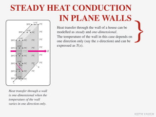
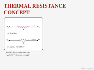
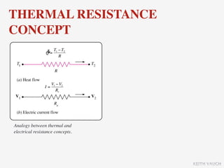
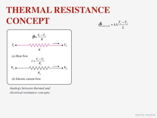
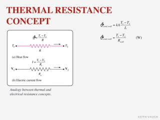
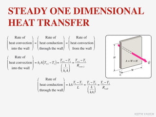
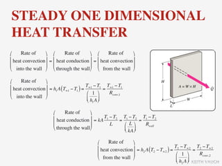
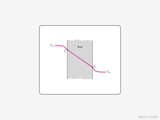
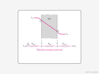
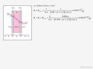
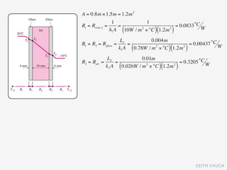
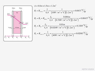
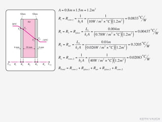
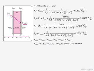
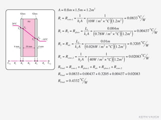
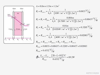
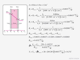
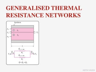
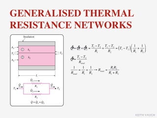
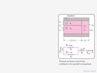
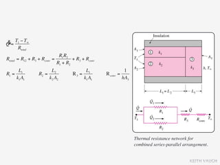
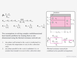
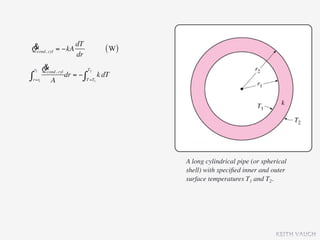
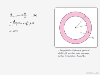
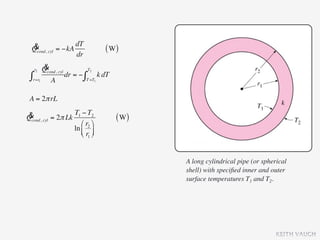
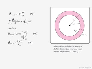
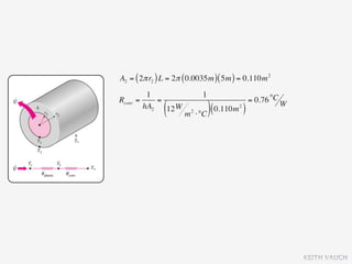
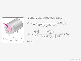
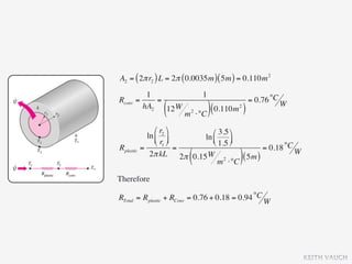
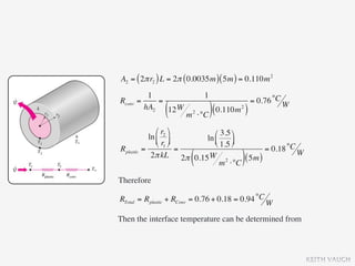
Definition and Requirements
Types of Heat Exchangers
The Overall Heat Transfer Coefficient
The Convection Heat Transfer Coefficients—Forced Convection
Heat Exchanger Analysis
Heat Exchanger Design and Performance Analysis
Obtain average velocity from a knowledge of velocity profile, and average temperature from a knowledge of temperature profile in internal flow.
Have a visual understanding of different flow regions in internal flow, and calculate hydrodynamic and thermal entry lengths.
Analyze heating and cooling of a fluid flowing in a tube under constant surface temperature and constant surface heat flux conditions, and work with the logarithmic mean temperature difference.
Obtain analytic relations for the velocity profile, pressure drop, friction factor, and Nusselt number in fully developed laminar flow.
Determine the friction factor and Nusselt number in fully developed turbulent flow using empirical relations, and calculate the heat transfer rate.
One dim, steady-state, heat conduction_with_heat_generationtmuliya
This file contains slides on One-dimensional, steady-state heat conduction with heat generation.
The slides were prepared while teaching Heat Transfer course to the M.Tech. students in Mechanical Engineering Dept. of St. Joseph Engineering College, Vamanjoor, Mangalore, India, during Sept. – Dec. 2010.
It is hoped that these Slides will be useful to teachers, students, researchers and professionals working in this field.
Solution Manual – Heat and Mass Transfer: Fundamentals and Application, 5th e...kl kl
Solution Manual – Heat and Mass Transfer: Fundamentals and Application, 5th edition
Author: Yunus A. Cengel, Afshin J. Ghajar
Publisher: McGraw-Hill Education
ISBN of textbook: 978-007-339818-1
This file contains slides on One-dimensional, steady state heat conduction without heat generation. The slides were prepared while teaching Heat Transfer course to the M.Tech. students.
Topics covered: Plane slab - composite slabs – contact resistance – cylindrical Systems – composite cylinders - spherical systems – composite spheres - critical thickness of insulation – optimum thickness – systems with variable thermal conductivity
This chapter contains:-.
Analytical Methods of two dimensional steady state heat conduction
Finite difference Method application on two dimensional steady state heat conduction.
Finite difference method on irregular shape of a system
SSL8 Mass & Energy Analysis of Control SystemsKeith Vaugh
Conservation of mass
Mass and volume flow rates
Mass balance for a steady flow process
Mass balance for incompressible flow
Flow work and the energy of a flowing fluid
Energy transport by mass
Energy analysis of steady flow systems
Steady flow engineering devices
Nozzles and diffusers
Turbines and compressors
Throttling valves
Mixing chambers and heat exchangers
Pipe and duct flow
Energy analysis of unsteady flow processes
GATE Mechanical Engineering notes on Heat Transfer. Use these notes as a preparation for GATE Mechanical Engineering and other engineering competitive exams. For full course visit https://mindvis.in/courses/gate-2018-mechanical-engineering-online-course or call 9779434433.
Heat Conduction with thermal heat generation.pptxBektu Dida
Heat Conduction analysis is done in one dimensional steady state heat conduction considering internal heat generation per unit volume on plane and radial walls. Examples are directly taken from textbooks.
The second law of thermodynamics is explored in this lecture. Topics covered include:
Introduction to the second law
Thermal energy reservoirs
Heat engines
Thermal efficiency
The 2nd law: Kelvin-Planck statement
Refrigerators and heat pumps
Coefficient of performance (COP)
The 2nd law: Clasius statement
Perpetual motion machines
Reversible and irreversible processes
Irreversibility's, Internal and externally reversible processes
The Carnot cycle
The reversed Carnot cycle
The Carnot principles
The thermodynamic temperature scale
The Carnot heat engine
The quality of energy
The Carnot refrigerator and heat pump
Mass flow and energy analysis of control systems is the focus of this lecture
Conservation of mass
Mass and volume flow rates
Mass balance for a steady flow process
Mass balance for incompressible flow
Flow work and the energy of a flowing fluid
his lecture examines both work and energy in closed systems and categorises the different types of closed systems that will be encountered.
Moving boundary work
Boundary work for an isothermal process
Boundary work for a constant-pressure process
Boundary work for a polytropic process
Energy balance for closed systems
Energy balance for a constant-pressure expansion or compression process
Specific heats
Constant-pressure specific heat, cp
Constant-volume specific heat, cv
Internal energy, enthalpy and specific heats of ideal gases
Energy balance for a constant-pressure expansion or compression process
Internal energy, enthalpy and specific heats of incompressible substances (Solids and liquids)
Identifying the correct properties of a substance is of vital importance. Many of these properties are distilled from property tables. This lecture addresses how to identify these properties.
Pure substance
Phases of a pure substance
Phase change processes of pure substances
Compressed liquid, Saturated liquid, Saturated vapor, Superheated vapor Saturated temperature and Satuated pressure
Property diagrams for phase change processes
The T-v diagram, The P-v diagram, The P-T diagram, The P-v-T diagram
Property tables
Enthalpy
Saturated liquid, Saturated vapor, Saturated liquid vapor mixture, Superheated vapor, compressed liquid
Reference state and Reference values
The ideal gas equation of state
Is water vapor an ideal gas?
Lecture covering the basic concepts required for the module:
Systems and control volumes
Properties of a system
Density and specific gravity
State and equilibrium
The state postulate
Processes and cycles
The state-flow process
Temperature and the zeroth law of thermodynamics
Temperature scales
Pressure
Variation of pressure with depths
2024.06.01 Introducing a competency framework for languag learning materials ...Sandy Millin
http://sandymillin.wordpress.com/iateflwebinar2024
Published classroom materials form the basis of syllabuses, drive teacher professional development, and have a potentially huge influence on learners, teachers and education systems. All teachers also create their own materials, whether a few sentences on a blackboard, a highly-structured fully-realised online course, or anything in between. Despite this, the knowledge and skills needed to create effective language learning materials are rarely part of teacher training, and are mostly learnt by trial and error.
Knowledge and skills frameworks, generally called competency frameworks, for ELT teachers, trainers and managers have existed for a few years now. However, until I created one for my MA dissertation, there wasn’t one drawing together what we need to know and do to be able to effectively produce language learning materials.
This webinar will introduce you to my framework, highlighting the key competencies I identified from my research. It will also show how anybody involved in language teaching (any language, not just English!), teacher training, managing schools or developing language learning materials can benefit from using the framework.
Acetabularia Information For Class 9 .docxvaibhavrinwa19
Acetabularia acetabulum is a single-celled green alga that in its vegetative state is morphologically differentiated into a basal rhizoid and an axially elongated stalk, which bears whorls of branching hairs. The single diploid nucleus resides in the rhizoid.
A Strategic Approach: GenAI in EducationPeter Windle
Artificial Intelligence (AI) technologies such as Generative AI, Image Generators and Large Language Models have had a dramatic impact on teaching, learning and assessment over the past 18 months. The most immediate threat AI posed was to Academic Integrity with Higher Education Institutes (HEIs) focusing their efforts on combating the use of GenAI in assessment. Guidelines were developed for staff and students, policies put in place too. Innovative educators have forged paths in the use of Generative AI for teaching, learning and assessments leading to pockets of transformation springing up across HEIs, often with little or no top-down guidance, support or direction.
This Gasta posits a strategic approach to integrating AI into HEIs to prepare staff, students and the curriculum for an evolving world and workplace. We will highlight the advantages of working with these technologies beyond the realm of teaching, learning and assessment by considering prompt engineering skills, industry impact, curriculum changes, and the need for staff upskilling. In contrast, not engaging strategically with Generative AI poses risks, including falling behind peers, missed opportunities and failing to ensure our graduates remain employable. The rapid evolution of AI technologies necessitates a proactive and strategic approach if we are to remain relevant.
Welcome to TechSoup New Member Orientation and Q&A (May 2024).pdfTechSoup
In this webinar you will learn how your organization can access TechSoup's wide variety of product discount and donation programs. From hardware to software, we'll give you a tour of the tools available to help your nonprofit with productivity, collaboration, financial management, donor tracking, security, and more.
1. STEADY HEAT
CONDUCTION
Lecture 4
Keith Vaugh BEng (AERO) MEng
Reference text: Chapter 17 - Fundamentals of Thermal-Fluid Sciences, 3rd Edition
Yunus A. Cengel, Robert H. Turner, John M. Cimbala
McGraw-Hill, 2008
KEITH VAUGH
3. OBJECTIVES
Understand the concept of thermal resistance and its
limitations, and develop thermal resistance networks
for practical heat conduction problems }
KEITH VAUGH
4. OBJECTIVES
Understand the concept of thermal resistance and its
limitations, and develop thermal resistance networks
for practical heat conduction problems
Solve steady conduction problems that involve
}
multilayer rectangular, cylindrical, or spherical
geometries
KEITH VAUGH
5. OBJECTIVES
Understand the concept of thermal resistance and its
limitations, and develop thermal resistance networks
for practical heat conduction problems
Solve steady conduction problems that involve
}
multilayer rectangular, cylindrical, or spherical
geometries
Develop an intuitive understanding of thermal contact
resistance, and circumstances under which it may be
significant
KEITH VAUGH
6. OBJECTIVES
Understand the concept of thermal resistance and its
limitations, and develop thermal resistance networks
for practical heat conduction problems
Solve steady conduction problems that involve
}
multilayer rectangular, cylindrical, or spherical
geometries
Develop an intuitive understanding of thermal contact
resistance, and circumstances under which it may be
significant
Identify applications in which insulation may actually
increase heat transfer
KEITH VAUGH
7. STEADY HEAT CONDUCTION
IN PLANE WALLS
Heat transfer through the wall of a house can be
modelled as steady and one-dimensional.
The temperature of the wall in this case depends on
one direction only (say the x-direction) and can be
expressed as T(x).
}
Heat transfer through a wall
is one-dimensional when the
temperature of the wall
varies in one direction only.
KEITH VAUGH
8. STEADY HEAT CONDUCTION
IN PLANE WALLS
Heat transfer through the wall of a house can be
modelled as steady and one-dimensional.
The temperature of the wall in this case depends on
one direction only (say the x-direction) and can be
expressed as T(x).
}
⎛ Rate of ⎞ ⎛ Rate of ⎞ ⎛ Rate of change ⎞
⎜ heat transfer ⎟ − ⎜ heat transfer ⎟ = ⎜ of the energy ⎟
⎜ ⎟ ⎜ ⎟ ⎜ ⎟
⎝ into the wall⎠ ⎝ out of the wall⎠ ⎝ of the wall ⎠
Heat transfer through a wall
is one-dimensional when the
temperature of the wall
varies in one direction only.
KEITH VAUGH
9. STEADY HEAT CONDUCTION
IN PLANE WALLS
Heat transfer through the wall of a house can be
modelled as steady and one-dimensional.
The temperature of the wall in this case depends on
one direction only (say the x-direction) and can be
expressed as T(x).
}
⎛ Rate of ⎞ ⎛ Rate of ⎞ ⎛ Rate of change ⎞
⎜ heat transfer ⎟ − ⎜ heat transfer ⎟ = ⎜ of the energy ⎟
⎜ ⎟ ⎜ ⎟ ⎜ ⎟
⎝ into the wall⎠ ⎝ out of the wall⎠ ⎝ of the wall ⎠
& − Qout = dEwall
Qin &
dt
Heat transfer through a wall
is one-dimensional when the
temperature of the wall
varies in one direction only.
KEITH VAUGH
10. STEADY HEAT CONDUCTION
IN PLANE WALLS
Heat transfer through the wall of a house can be
modelled as steady and one-dimensional.
The temperature of the wall in this case depends on
one direction only (say the x-direction) and can be
expressed as T(x).
}
⎛ Rate of ⎞ ⎛ Rate of ⎞ ⎛ Rate of change ⎞
⎜ heat transfer ⎟ − ⎜ heat transfer ⎟ = ⎜ of the energy ⎟
⎜ ⎟ ⎜ ⎟ ⎜ ⎟
⎝ into the wall⎠ ⎝ out of the wall⎠ ⎝ of the wall ⎠
& − Qout = dEwall
Qin &
dt
In steady operation, the rate of heat transfer
Heat transfer through a wall
through the wall is constant.
is one-dimensional when the
temperature of the wall
varies in one direction only. & dT Fourier’s law of
Qcond,wall = −kA (W)
dx heat conduction
KEITH VAUGH
12. Under steady conditions, the
temperature distribution in a
plane wall is a straight line:
dT/dx = const.
KEITH VAUGH
13. & dT
Qcond,wall = −kA
dx
Under steady conditions, the
temperature distribution in a
plane wall is a straight line:
dT/dx = const.
KEITH VAUGH
14. & dT
Qcond,wall = −kA
dx
&
L T2
∫ Qcond,wall dx = − ∫ kA dT
x=0 T =T1
Under steady conditions, the
temperature distribution in a
plane wall is a straight line:
dT/dx = const.
KEITH VAUGH
15. & dT
Qcond,wall = −kA
dx
&
L T2
∫ Qcond,wall dx = − ∫ kA dT
x=0 T =T1
& T1 − T2
Qcond,wall = kA (W)
L
Under steady conditions, the
temperature distribution in a
plane wall is a straight line:
dT/dx = const.
KEITH VAUGH
16. & dT
Qcond,wall = −kA
dx
&
L T2
∫ Qcond,wall dx = − ∫ kA dT
x=0 T =T1
& T1 − T2
Qcond,wall = kA (W)
L
The rate of heat conduction through a plane wall is
proportional to the average thermal conductivity, the
wall area, and the temperature difference, but is
inversely proportional to the wall thickness.
Under steady conditions, the Once the rate of heat conduction is available, the
temperature distribution in a temperature T(x) at any location x can be determined
plane wall is a straight line:
dT/dx = const.
by replacing T2 by T, and L by x.
KEITH VAUGH
18. THERMAL RESISTANCE
CONCEPT
& T −T
Q= 1 2
R
V1 − V2
I=
Re
Analogy between thermal and
electrical resistance concepts.
KEITH VAUGH
19. THERMAL RESISTANCE
CONCEPT &
Q = kA
T −T
cond,wall
1 2
L
& T −T
Q= 1 2
R
V1 − V2
I=
Re
Analogy between thermal and
electrical resistance concepts.
KEITH VAUGH
20. THERMAL RESISTANCE
CONCEPT &
Q = kA
T −T
cond,wall
1 2
L
& T −T & T1 − T2
Q= 1 2 Qcond,wall = (W)
R Rwall
V1 − V2
I=
Re
Analogy between thermal and
electrical resistance concepts.
KEITH VAUGH
21. THERMAL RESISTANCE
CONCEPT &
Q = kA
T −T
cond,wall
1 2
L
& T −T & T1 − T2
Q= 1 2 Qcond,wall = (W)
R Rwall
Conduction resistance of the wall:
Thermal resistance of the wall against heat
V1 − V2 conduction.
I=
Re
L
Rwall =
kA
(°C W )
Thermal resistance of a medium depends on
Analogy between thermal and the geometry and the thermal properties of
electrical resistance concepts. the medium.
KEITH VAUGH
22. THERMAL RESISTANCE
CONCEPT &
Q = kA
T −T
cond,wall
1 2
L
& T −T & T1 − T2
Q= 1 2 Qcond,wall = (W)
R Rwall
Conduction resistance of the wall:
Thermal resistance of the wall against heat
V1 − V2 conduction.
I=
Re
L
Rwall =
kA
(°C W )
Thermal resistance of a medium depends on
Analogy between thermal and the geometry and the thermal properties of
electrical resistance concepts. the medium.
rate of heat transfer → electric current V1 − V2 Re = L σ A
thermal resistance → electrical resistance I= e
Re
temperature difference → voltage difference Electrical resistance
KEITH VAUGH
24. & Newton’s law
Qconv = hAs (Ts − T∞ )
of cooling
Schematic for convection resistance at a surface.
KEITH VAUGH
25. & Newton’s law
Qconv = hAs (Ts − T∞ )
of cooling
& = Ts − T∞
Qconv (W)
Rconv
Convection resistance of the surface:
Thermal resistance of the surface against heat
convection.
1
Rwall =
hAs
(°C W )
Schematic for convection resistance at a surface.
When the convection heat transfer coefficient is very large (h → ∞), the
convection resistance becomes zero and Ts ≈ T.
That is, the surface offers no resistance to convection, and thus it does
not slow down the heat transfer process.
This situation is approached in practice at surfaces where boiling and
condensation occur.
KEITH VAUGH
28. & = εσ As Ts4 − Tsurr = hrad As (Ts − Tsurr ) = Ts − Tsurr
Qrad ( 4
) Rrad
Radiation resistance of the surface:
Thermal resistance of the surface against heat radiation.
Schematic for convection
and radiation resistances at
a surface. KEITH VAUGH
29. & = εσ As Ts4 − Tsurr = hrad As (Ts − Tsurr ) = Ts − Tsurr
Qrad ( 4
) Rrad
Radiation resistance of the surface:
Thermal resistance of the surface against heat radiation.
1
Rrad =
hrad As
(K W )
Schematic for convection
and radiation resistances at
a surface. KEITH VAUGH
30. & = εσ As Ts4 − Tsurr = hrad As (Ts − Tsurr ) = Ts − Tsurr
Qrad ( 4
) Rrad
Radiation resistance of the surface:
Thermal resistance of the surface against heat radiation.
1
Rrad =
hrad As
( K
W )
&
Qrad
hrad =
As (Ts − Tsurr )
( )
= εσ Ts2 + Tsurr (Ts + Tsurr )
2
(W m ⋅ K )
2 Note: K (Kelvins), for
radiation analysis Ts and
Tsurr must be in Kelvins
Schematic for convection
and radiation resistances at
a surface. KEITH VAUGH
31. & = εσ As Ts4 − Tsurr = hrad As (Ts − Tsurr ) = Ts − Tsurr
Qrad ( 4
) Rrad
Radiation resistance of the surface:
Thermal resistance of the surface against heat radiation.
1
Rrad =
hrad As
( K
W )
&
Qrad
hrad =
As (Ts − Tsurr )
( )
= εσ Ts2 + Tsurr (Ts + Tsurr )
2
(W m ⋅ K )
2 Note: K (Kelvins), for
radiation analysis Ts and
Tsurr must be in Kelvins
When Tsurr ≈ T∞
hcombined = hconv + hrad
Combined heat transfer coefficient
Schematic for convection
and radiation resistances at
a surface. KEITH VAUGH
33. STEADY ONE DIMENSIONAL
HEAT TRANSFER
⎛ Rate of ⎞ ⎛ Rate of ⎞ ⎛ Rate of ⎞
⎜ heat convection ⎟ = ⎜ heat conduction ⎟ = ⎜ heat convection ⎟
⎜ ⎟ ⎜ ⎟ ⎜ ⎟
⎝ into the wall ⎠ ⎝ through the wall⎠ ⎝ from the wall ⎠
KEITH VAUGH
34. STEADY ONE DIMENSIONAL
HEAT TRANSFER
⎛ Rate of ⎞ ⎛ Rate of ⎞ ⎛ Rate of ⎞
⎜ heat convection ⎟ = ⎜ heat conduction ⎟ = ⎜ heat convection ⎟
⎜ ⎟ ⎜ ⎟ ⎜ ⎟
⎝ into the wall ⎠ ⎝ through the wall⎠ ⎝ from the wall ⎠
⎛ Rate of ⎞
⎜ heat convection ⎟ = h A (T − T ) = T∞1 − T1 = T∞1 − T1
1 ∞1 1
⎜ ⎟ ⎛ 1 ⎞ Rconv,1
⎝ into the wall ⎠ ⎜ h A ⎟
⎝ 1 ⎠
KEITH VAUGH
35. STEADY ONE DIMENSIONAL
HEAT TRANSFER
⎛ Rate of ⎞ ⎛ Rate of ⎞ ⎛ Rate of ⎞
⎜ heat convection ⎟ = ⎜ heat conduction ⎟ = ⎜ heat convection ⎟
⎜ ⎟ ⎜ ⎟ ⎜ ⎟
⎝ into the wall ⎠ ⎝ through the wall⎠ ⎝ from the wall ⎠
⎛ Rate of ⎞
⎜ heat convection ⎟ = h A (T − T ) = T∞1 − T1 = T∞1 − T1
1 ∞1 1
⎜ ⎟ ⎛ 1 ⎞ Rconv,1
⎝ into the wall ⎠ ⎜ h A ⎟
⎝ 1 ⎠
⎛ Rate of ⎞
⎜ heat conduction ⎟ = kA T1 − T2 = T1 − T2 = T1 − T2
⎜ ⎟ L ⎛ L ⎞ Rwall
⎝ through the wall⎠ ⎜ ⎟
⎝ kA ⎠
KEITH VAUGH
36. STEADY ONE DIMENSIONAL
HEAT TRANSFER
⎛ Rate of ⎞ ⎛ Rate of ⎞ ⎛ Rate of ⎞
⎜ heat convection ⎟ = ⎜ heat conduction ⎟ = ⎜ heat convection ⎟
⎜ ⎟ ⎜ ⎟ ⎜ ⎟
⎝ into the wall ⎠ ⎝ through the wall⎠ ⎝ from the wall ⎠
⎛ Rate of ⎞
⎜ heat convection ⎟ = h A (T − T ) = T∞1 − T1 = T∞1 − T1
1 ∞1 1
⎜ ⎟ ⎛ 1 ⎞ Rconv,1
⎝ into the wall ⎠ ⎜ h A ⎟
⎝ 1 ⎠
⎛ Rate of ⎞
⎜ heat conduction ⎟ = kA T1 − T2 = T1 − T2 = T1 − T2
⎜ ⎟ L ⎛ L ⎞ Rwall
⎝ through the wall⎠ ⎜ ⎟
⎝ kA ⎠
⎛ Rate of ⎞
⎜ heat convection ⎟ = h A (T − T ) = T2 − T∞2 = T2 − T∞2
2 2 ∞2
⎜ ⎟ ⎛ 1 ⎞ Rconv,2
⎝ from the wall ⎠ ⎜ h A ⎟
⎝ 2 ⎠ KEITH VAUGH
43. &= T∞1 − T∞2
Q
Rtotal
Thermal resistance network
1 L 1
Rtotal = Rconv,1 + Rwall + Rconv,2 = + +
h1 A kA h2 A
(°C W )
KEITH VAUGH
44. The temperature drop across a layer is
proportional to its thermal resistance.
KEITH VAUGH
45. The ratio of temperature drop to thermal resistance
across the layer is proportional, therefore:
&
ΔT = QR (°C )
The temperature drop across a layer is
proportional to its thermal resistance.
KEITH VAUGH
46. The ratio of temperature drop to thermal resistance
across the layer is proportional, therefore:
&
ΔT = QR (°C )
Heat transfer can be expressed in a similar manner
to Newtons Law of cooling:
&
Q = UAΔT ( W)
U overall heat transfer coefficient
The temperature drop across a layer is
proportional to its thermal resistance.
KEITH VAUGH
47. The ratio of temperature drop to thermal resistance
across the layer is proportional, therefore:
&
ΔT = QR (°C )
Heat transfer can be expressed in a similar manner
to Newtons Law of cooling:
&
Q = UAΔT ( W)
U overall heat transfer coefficient
Comparing Q &= T∞1 − T∞2 and Q = UAΔT , reveals
&
Rtotal
1
UA =
Rtotal
(°C
K)
The temperature drop across a layer is
proportional to its thermal resistance.
KEITH VAUGH
48. The ratio of temperature drop to thermal resistance
across the layer is proportional, therefore:
&
ΔT = QR (°C )
Heat transfer can be expressed in a similar manner
to Newtons Law of cooling:
&
Q = UAΔT ( W)
U overall heat transfer coefficient
Comparing Q &= T∞1 − T∞2 and Q = UAΔT , reveals
&
Rtotal
1
UA =
Rtotal
(°C
K)
The temperature drop across a layer is
Once Q is evaluated, the surface temperature T1
proportional to its thermal resistance.
can be determined from
KEITH VAUGH
49. The ratio of temperature drop to thermal resistance
across the layer is proportional, therefore:
&
ΔT = QR (°C )
Heat transfer can be expressed in a similar manner
to Newtons Law of cooling:
&
Q = UAΔT ( W)
U overall heat transfer coefficient
Comparing Q &= T∞1 − T∞2 and Q = UAΔT , reveals
&
Rtotal
1
UA =
Rtotal
(°C
K )
The temperature drop across a layer is
Once Q is evaluated, the surface temperature T1
proportional to its thermal resistance.
can be determined from
&= T∞1 − T1 = T∞1 − T1
Q
Rconv,1 ⎛ 1 ⎞
⎜ h A ⎟
⎝ 1 ⎠
KEITH VAUGH
50. MULTILAYER PLANE
WALLS
The thermal resistance
network for heat transfer
through a two-layer plane
wall subjected to
convection on both sides.
KEITH VAUGH
51. MULTILAYER PLANE
WALLS
The thermal resistance
network for heat transfer
through a two-layer plane
wall subjected to
convection on both sides.
&= T∞1 − T∞2
Q
Rtotal
KEITH VAUGH
52. MULTILAYER PLANE
WALLS
The thermal resistance
network for heat transfer
through a two-layer plane
wall subjected to
convection on both sides.
&= T∞1 − T∞2
Q
Rtotal
1 L1 L2 1
Rtotal = Rconv,1 + Rwall,1 + Rwall,2 + Rconv,2 = + + +
h1 A k1 A k2 A h2 A
(°C W )
KEITH VAUGH
54. An unknown surface temperature Tj on any surface or
interface j can be calculate when T∞1 and T∞2 are given
and the rate heat transfer is known
T − Tj where Ti is a known temperature at
&= i
Q location i and Rtotal, i-j is the total thermal
Rtotal, i− j
resistances between location i and j.
KEITH VAUGH
55. An unknown surface temperature Tj on any surface or
interface j can be calculate when T∞1 and T∞2 are given
and the rate heat transfer is known
T − Tj where Ti is a known temperature at
&= i
Q location i and Rtotal, i-j is the total thermal
Rtotal, i− j
resistances between location i and j.
& T∞1 − T∞2 T∞1 − T∞2
Q= =
Rconv, 1 + Rwall, 1 ⎛ 1 ⎞ ⎛ L1 ⎞
⎜ h A ⎟ + ⎜ k A ⎟
⎝ 1 ⎠ ⎝ 1 ⎠
KEITH VAUGH
56. An unknown surface temperature Tj on any surface or
interface j can be calculate when T∞1 and T∞2 are given
and the rate heat transfer is known
T − Tj where Ti is a known temperature at
&= i
Q location i and Rtotal, i-j is the total thermal
Rtotal, i− j
resistances between location i and j.
& T∞1 − T∞2 T∞1 − T∞2
Q= =
Rconv, 1 + Rwall, 1 ⎛ 1 ⎞ ⎛ L1 ⎞
⎜ h A ⎟ + ⎜ k A ⎟
⎝ 1 ⎠ ⎝ 1 ⎠
To find T1 : &= T∞1 − T1
Q
Rconv, 1
& T∞1 − T2
To find T2 : Q=
Rconv, 1 + Rwall, 1
To find T3 : &= T3 − T∞2
Q
Rconv, 2
Refer to pages 659-663 in text book KEITH VAUGH
57. QUESTION
A double pane glass window 0.8 m high and 1.5 m
wide consisting of two 4 mm thick layers of glass
each having a thermal conductivity k = 0.78
W·m-1·K-1 and separated by a 10 mm wide stagnant
}
air space is used in a building. Determine the steady
rate of heat transfer through this window and the
temperature of its inner surface for a day during
which the room is maintained at 20°C and the outside
temperature is -10°C. Assume the heat transfer
coefficients on the inner and outer surfaces of the
window to be h1 = 10 W/m2 °C and h2 = 40 W·m-2·
°C-1, which includes the effects of radiation.
KEITH VAUGH
58. Question marked approximately as:
Identification of problem: 0-39% (39% band)
Formulation of problem: 40-69% (29% band)
Solution of problem: 70-100% (30% band)
KEITH VAUGH
60. ASSUMPTIONS
Heat transfer through the mediums is steady
Heat transfer is one dimensional
Thermal conductivity is constant
KEITH VAUGH
61. ASSUMPTIONS
Heat transfer through the mediums is steady
Heat transfer is one dimensional
Thermal conductivity is constant
KEITH VAUGH
62. ASSUMPTIONS ANALYSIS
Heat transfer through the mediums is steady A double pane window is considered. The rate of
Heat transfer is one dimensional heat transfer through the window and the inner
Thermal conductivity is constant surface temperature are to be determined
The diagram illustrates this problem. We do not
know the values of T2, T3 therefore must employ
the concept of thermal resistance,
KEITH VAUGH
63. ASSUMPTIONS ANALYSIS
Heat transfer through the mediums is steady A double pane window is considered. The rate of
Heat transfer is one dimensional heat transfer through the window and the inner
Thermal conductivity is constant surface temperature are to be determined
The diagram illustrates this problem. We do not
know the values of T2, T3 therefore must employ
the concept of thermal resistance,
&= ΔTmediums L
Q where, Rmediums =
ΔRmediums kA
The thermal resistance network comprises of 5
elements, Ri, Ro, representing the inner and outer
elements, R1, R3, representing the inner and outer
glass panes, and R2 represents the Air cavity. This
problem comprises both conduction and
convection.
KEITH VAUGH
66. A = 0.8m × 1.5m = 1.2m 2
1 1
Ri = Rconv,1 = = = 0.0833 °C W
( 2
)(
h1 A 10W / m × °C 1.2m )
2
KEITH VAUGH
67. A = 0.8m × 1.5m = 1.2m 2
1 1
Ri = Rconv,1 = = = 0.0833 °C W
( 2
)(
h1 A 10W / m × °C 1.2m 2
)
L1 0.004m
R1 = R3 = Rglass = = = 0.00437 °C W
k1 A ( )( )
0.78W / m 2 × °C 1.2m 2
KEITH VAUGH
68. A = 0.8m × 1.5m = 1.2m 2
1 1
Ri = Rconv,1 = = = 0.0833 °C W
( 2
)(
h1 A 10W / m × °C 1.2m 2
)
L1 0.004m
R1 = R3 = Rglass = = = 0.00437 °C W
k1 A ( )(
0.78W / m 2 × °C 1.2m 2 )
L2 0.01m
R2 = Rair = = = 0.3205 °C W
k2 A ( 2
0.026W / m × °C 1.2m 2
)( )
KEITH VAUGH
69. A = 0.8m × 1.5m = 1.2m 2
1 1
Ri = Rconv,1 = = = 0.0833 °C W
( 2
)(
h1 A 10W / m × °C 1.2m 2
)
L1 0.004m
R1 = R3 = Rglass = = = 0.00437 °C W
k1 A ( )(
0.78W / m 2 × °C 1.2m 2 )
L2 0.01m
R2 = Rair = = = 0.3205 °C W
k2 A ( 2
0.026W / m × °C 1.2m 2
)( )
1 1
Ro = Rconv,2 = = = 0.02083 °C W
h2 A ( )(
40W / m 2 × °C 1.2m 2 )
KEITH VAUGH
70. A = 0.8m × 1.5m = 1.2m 2
1 1
Ri = Rconv,1 = = = 0.0833 °C W
(2
h1 A 10W / m × °C 1.2m 2
)( )
L1 0.004m
R1 = R3 = Rglass = = = 0.00437 °C W
k1 A (
0.78W / m 2 × °C 1.2m 2 )( )
L2 0.01m
R2 = Rair = = = 0.3205 °C W
k2 A ( 2
0.026W / m × °C 1.2m 2
)( )
1 1
Ro = Rconv,2 = = = 0.02083 °C W
h2 A (
40W / m 2 × °C 1.2m 2)( )
RTotal = Rconv,1 + Rglass,1 + Rair + Rglass,2 + Rconv,2
KEITH VAUGH
71. A = 0.8m × 1.5m = 1.2m 2
1 1
Ri = Rconv,1 = = = 0.0833 °C W
(2
h1 A 10W / m × °C 1.2m 2
)( )
L1 0.004m
R1 = R3 = Rglass = = = 0.00437 °C W
k1 A (
0.78W / m 2 × °C 1.2m 2 )( )
L2 0.01m
R2 = Rair = = = 0.3205 °C W
k2 A ( 2
0.026W / m × °C 1.2m 2
)( )
1 1
Ro = Rconv,2 = = = 0.02083 °C W
h2 A (
40W / m 2 × °C 1.2m 2)( )
RTotal = Rconv,1 + Rglass,1 + Rair + Rglass,2 + Rconv,2
RTotal = 0.0833 + 0.00437 + 0.3205 + 0.00437 + 0.02083
KEITH VAUGH
72. A = 0.8m × 1.5m = 1.2m 2
1 1
Ri = Rconv,1 = = = 0.0833 °C W
(2
h1 A 10W / m × °C 1.2m 2
)( )
L1 0.004m
R1 = R3 = Rglass = = = 0.00437 °C W
k1 A (
0.78W / m 2 × °C 1.2m 2 )( )
L2 0.01m
R2 = Rair = = = 0.3205 °C W
k2 A ( 2
0.026W / m × °C 1.2m 2
)( )
1 1
Ro = Rconv,2 = = = 0.02083 °C W
h2 A (
40W / m 2 × °C 1.2m 2)( )
RTotal = Rconv,1 + Rglass,1 + Rair + Rglass,2 + Rconv,2
RTotal = 0.0833 + 0.00437 + 0.3205 + 0.00437 + 0.02083
RTotal = 0.4332 °C W
KEITH VAUGH
73. A = 0.8m × 1.5m = 1.2m 2
1 1
Ri = Rconv,1 = = = 0.0833 °C W
(2
h1 A 10W / m × °C 1.2m 2
)( )
L1 0.004m
R1 = R3 = Rglass = = = 0.00437 °C W
k1 A (
0.78W / m 2 × °C 1.2m 2 )( )
L2 0.01m
R2 = Rair = = = 0.3205 °C W
k2 A ( 2
0.026W / m × °C 1.2m 2
)( )
1 1
Ro = Rconv,2 = = = 0.02083 °C W
h2 A (
40W / m 2 × °C 1.2m 2)( )
RTotal = Rconv,1 + Rglass,1 + Rair + Rglass,2 + Rconv,2
RTotal = 0.0833 + 0.00437 + 0.3205 + 0.00437 + 0.02083
RTotal = 0.4332 °C W
Q ⎣ 20 − ( −10 ) ⎤ °C = 69.2W
&= T∞1 − T∞2 = ⎡ ⎦
RTotal 0.4332 °C W
KEITH VAUGH
74. A = 0.8m × 1.5m = 1.2m 2
1 1
Ri = Rconv,1 = = = 0.0833 °C W
(2
h1 A 10W / m × °C 1.2m 2
)( )
L1 0.004m
R1 = R3 = Rglass = = = 0.00437 °C W
k1 A (
0.78W / m 2 × °C 1.2m 2 )( )
L2 0.01m
R2 = Rair = = = 0.3205 °C W
k2 A ( 2
0.026W / m × °C 1.2m 2
)( )
1 1
Ro = Rconv,2 = = = 0.02083 °C W
h2 A (
40W / m 2 × °C 1.2m 2 )( )
RTotal = Rconv,1 + Rglass,1 + Rair + Rglass,2 + Rconv,2
RTotal = 0.0833 + 0.00437 + 0.3205 + 0.00437 + 0.02083
RTotal = 0.4332 °C W
Q ⎣ 20 − ( −10 ) ⎤ °C = 69.2W
&= T∞1 − T∞2 = ⎡ ⎦
RTotal 0.4332 °C W
& (
T1 = T∞1 − QRconv,1 = 20 − ( 69.2W ) 0.0833 °C W = 14.2°C )
KEITH VAUGH
76. THERMAL CONTACT
RESISTANCE
When two such surfaces are pressed against each other,
the peaks form good material contact but the valleys form
voids filled with air. }
KEITH VAUGH
77. THERMAL CONTACT
RESISTANCE
When two such surfaces are pressed against each other,
the peaks form good material contact but the valleys form
voids filled with air. }
These numerous air gaps of varying sizes act as
insulation because of the low thermal conductivity of air.
KEITH VAUGH
78. THERMAL CONTACT
RESISTANCE
When two such surfaces are pressed against each other,
the peaks form good material contact but the valleys form
voids filled with air. }
These numerous air gaps of varying sizes act as
insulation because of the low thermal conductivity of air.
Thus, an interface offers some resistance to heat transfer,
and this resistance per unit interface area is called the
thermal contact resistance, Rc.
KEITH VAUGH
79. Temperature distribution and heat flow lines along
two solid plates pressed against each other for the
case of perfect and imperfect contact.
KEITH VAUGH
80. Temperature distribution and heat flow lines along
two solid plates pressed against each other for the
case of perfect and imperfect contact.
KEITH VAUGH
81. The value of thermal contact resistance depends on:
✓ surface roughness,
✓ material properties,
✓ temperature and pressure at the interface
✓ type of fluid trapped at the interface.
KEITH VAUGH
82. The value of thermal contact resistance depends on:
✓ surface roughness,
✓ material properties,
✓ temperature and pressure at the interface
✓ type of fluid trapped at the interface.
& & &
Q = Qcontact + Qgap
KEITH VAUGH
83. The value of thermal contact resistance depends on:
✓ surface roughness,
✓ material properties,
✓ temperature and pressure at the interface
✓ type of fluid trapped at the interface.
& & &
Q = Qcontact + Qgap
&
Q = hc AΔTinterface hc thermal contact conductance
KEITH VAUGH
84. The value of thermal contact resistance depends on:
✓ surface roughness,
✓ material properties,
✓ temperature and pressure at the interface
✓ type of fluid trapped at the interface.
& & &
Q = Qcontact + Qgap
&
Q = hc AΔTinterface hc thermal contact conductance
&
⎛ Q ⎞
⎜ A ⎟
⎝ ⎠
hc =
ΔTinterface (W m ⋅°C )
2
KEITH VAUGH
85. The value of thermal contact resistance depends on:
✓ surface roughness,
✓ material properties,
✓ temperature and pressure at the interface
✓ type of fluid trapped at the interface.
& & &
Q = Qcontact + Qgap
&
Q = hc AΔTinterface hc thermal contact conductance
&
⎛ Q ⎞
⎜ A ⎟
⎝ ⎠
hc =
ΔTinterface (W m ⋅°C )
2
1 ΔTinterface
Rc = =
hc &
⎛ Q ⎞
( m ⋅ °C W )
2
⎜ A ⎟
⎝ ⎠
KEITH VAUGH
86. The value of thermal contact resistance depends on:
✓ surface roughness,
✓ material properties,
✓ temperature and pressure at the interface
✓ type of fluid trapped at the interface.
& & &
Q = Qcontact + Qgap
&
Q = hc AΔTinterface hc thermal contact conductance
&
⎛ Q ⎞
⎜ A ⎟
⎝ ⎠
hc =
ΔTinterface (W m ⋅°C )
2
1 ΔTinterface
Rc = =
hc &
⎛ Q ⎞
( m ⋅ °C W )
2
⎜ A ⎟
⎝ ⎠
Thermal contact resistance is significant and can even dominate
the heat transfer for good heat conductors such as metals, but can
be disregarded for poor heat conductors such as insulations.
KEITH VAUGH
92. &= T1 − T∞
Q
Rtotal
R1 R2
Rtotal = R12 + R3 + Rconv = + R3 + Rconv
R1 + R2
L1 L2 L1 1
R1 = R2 = R3 = R conv =
k1 A1 k2 A2 k1 A1 hA3
Two assumptions in solving complex multidimensional
heat transfer problems by treating them as one-
dimensional using the thermal resistance network are:
1. Any plane wall normal to the x-axis is isothermal (i.e.
to assume the temperature to vary in the x-direction
only)
2. any plane parallel to the x-axis is adiabatic (i.e. to Thermal resistance network for
assume heat transfer to occur in the x-direction only) combined series-parallel arrangement.
KEITH VAUGH
94. HEAT CONDUCTION IN
CYLINDERS & SPHERES
Heat transfer through the pipe can be
modelled as steady and one-dimensional.
}
KEITH VAUGH
95. HEAT CONDUCTION IN
CYLINDERS & SPHERES
Heat transfer through the pipe can be
modelled as steady and one-dimensional.
The temperature of the pipe depends on one
}
direction only (the radial r-direction) and
can be expressed as T = T(r).
KEITH VAUGH
96. HEAT CONDUCTION IN
CYLINDERS & SPHERES
Heat transfer through the pipe can be
modelled as steady and one-dimensional.
The temperature of the pipe depends on one
}
direction only (the radial r-direction) and
can be expressed as T = T(r).
The temperature is independent of the
azimuthal angle or the axial distance.
KEITH VAUGH
97. HEAT CONDUCTION IN
CYLINDERS & SPHERES
Heat transfer through the pipe can be
modelled as steady and one-dimensional.
The temperature of the pipe depends on one
}
direction only (the radial r-direction) and
can be expressed as T = T(r).
The temperature is independent of the
azimuthal angle or the axial distance.
This situation is approximated in practice in
long cylindrical pipes and spherical
containers.
KEITH VAUGH
98. A long cylindrical pipe (or spherical
shell) with specified inner and outer
surface temperatures T1 and T2.
KEITH VAUGH
99. & cyl = −kA dT
Qcond, ( W)
dr
A long cylindrical pipe (or spherical
shell) with specified inner and outer
surface temperatures T1 and T2.
KEITH VAUGH
100. & cyl = −kA dT
Qcond, ( W)
dr
r2 &
Qcond, cyl T2
∫r=r1 A dr = − ∫T =T1 k dT
A long cylindrical pipe (or spherical
shell) with specified inner and outer
surface temperatures T1 and T2.
KEITH VAUGH
101. & cyl = −kA dT
Qcond, ( W)
dr
r2 &
Qcond, cyl T2
∫r=r1 A dr = − ∫T =T1 k dT
A = 2π rL
A long cylindrical pipe (or spherical
shell) with specified inner and outer
surface temperatures T1 and T2.
KEITH VAUGH
102. & cyl = −kA dT
Qcond, ( W)
dr
r2 &
Qcond, cyl T2
∫r=r1 A dr = − ∫T =T1 k dT
A = 2π rL
& cyl = 2π Lk T1 − T2
Qcond, ( W)
⎛ r2 ⎞
ln ⎜ ⎟
⎝ r1 ⎠
A long cylindrical pipe (or spherical
shell) with specified inner and outer
surface temperatures T1 and T2.
KEITH VAUGH
103. & cyl = −kA dT
Qcond, ( W)
dr
r2 &
Qcond, cyl T2
∫r=r1 A dr = − ∫T =T1 k dT
A = 2π rL
& cyl = 2π Lk T1 − T2
Qcond, ( W)
⎛ r2 ⎞
ln ⎜ ⎟
⎝ r1 ⎠
& cyl = T1 − T2
Qcond, ( W)
Rcyl
A long cylindrical pipe (or spherical
shell) with specified inner and outer
surface temperatures T1 and T2.
KEITH VAUGH
104. & cyl = −kA dT
Qcond, ( W)
dr
r2 &
Qcond, cyl T2
∫r=r1 A dr = − ∫T =T1 k dT
A = 2π rL
& cyl = 2π Lk T1 − T2
Qcond, ( W)
⎛ r2 ⎞
ln ⎜ ⎟
⎝ r1 ⎠
& cyl = T1 − T2
Qcond, ( W)
Rcyl
A long cylindrical pipe (or spherical
shell) with specified inner and outer
surface temperatures T1 and T2.
⎛ r2 ⎞ ⎛ outer radius ⎞
ln ⎜ ⎟ ln ⎜
⎝ r1 ⎠ ⎝ inner radius ⎟
⎠
Rcyl = =
2π Lk 2π × Length × Thermal conductivity
KEITH VAUGH
105. & cyl = −kA dT
Qcond, ( W)
dr
r2 &
Qcond, cyl T2
∫r=r1 A dr = − ∫T =T1 k dT
A = 2π rL
& cyl = 2π Lk T1 − T2
Qcond, ( W)
⎛ r2 ⎞
ln ⎜ ⎟
⎝ r1 ⎠
& cyl = T1 − T2
Qcond, ( W)
Rcyl
A long cylindrical pipe (or spherical
shell) with specified inner and outer
surface temperatures T1 and T2.
⎛ r2 ⎞ ⎛ outer radius ⎞
ln ⎜ ⎟ ln ⎜
⎝ r1 ⎠ ⎝ inner radius ⎟
⎠ Conduction resistance of
Rcyl = = the cylinder layer
2π Lk 2π × Length × Thermal conductivity
KEITH VAUGH
106. A spherical shell with specified inner and
outer surface temperatures T1 and T2.
KEITH VAUGH
107. A spherical shell with specified inner and
outer surface temperatures T1 and T2.
& sph = T1 − T2
Qcond,
Rsph
KEITH VAUGH
108. A spherical shell with specified inner and
outer surface temperatures T1 and T2.
& sph = T1 − T2
Qcond,
Rsph
r2 − r1 outer radius - inner radius
Rsph = =
2π r1r2 k 2π ( outer radius ) ( inner radius ) ( Thermal conductivity )
KEITH VAUGH
110. &= T∞1 − T∞2
Q
Rtotal
The thermal resistance network for a cylindrical
(or spherical) shell subjected to convection from
both the inner and the outer sides.
KEITH VAUGH
111. &= T∞1 − T∞2
Q
Rtotal
for a cylindrical layer
Rtotal = Rconv, 1 + Rcyl + Rconv, 2
⎛ r2 ⎞
ln ⎜ ⎟
1 ⎝ r1 ⎠ 1
= + +
( 2π r1L ) h1 2π Lk ( 2π r2 L ) h2
The thermal resistance network for a cylindrical
(or spherical) shell subjected to convection from
both the inner and the outer sides.
KEITH VAUGH
112. &= T∞1 − T∞2
Q
Rtotal
for a cylindrical layer
Rtotal = Rconv, 1 + Rcyl + Rconv, 2
⎛ r2 ⎞
ln ⎜ ⎟
1 ⎝ r1 ⎠ 1
= + +
( 2π r1L ) h1 2π Lk ( 2π r2 L ) h2
for a spherical layer
The thermal resistance network for a cylindrical Rtotal = Rconv, 1 + Rsph + Rconv,2
(or spherical) shell subjected to convection from 1 r −r 1
both the inner and the outer sides. = + 2 1 +
( ) ( )
4π r12 h1 4π r1r2 k 4π r22 h2
KEITH VAUGH
113. MULTILAYER CYLINDER &
SPHERES
The thermal resistance network for heat
transfer through a three-layered composite
cylinder subjected to convection on both
sides.
KEITH VAUGH
114. MULTILAYER CYLINDER &
SPHERES
The thermal resistance network for heat
transfer through a three-layered composite
cylinder subjected to convection on both
sides.
&= T∞1 − T∞2
Q
Rtotal
KEITH VAUGH
115. MULTILAYER CYLINDER &
SPHERES
The thermal resistance network for heat
transfer through a three-layered composite
cylinder subjected to convection on both
sides.
&= T∞1 − T∞2
Q
Rtotal
⎛ r3 ⎞ ⎛ r4 ⎞ ⎛ r2 ⎞
ln ⎜ ⎟ ln ⎜ ⎟ ln ⎜ ⎟
1 ⎝ r2 ⎠ ⎝ r3 ⎠ ⎝ r1 ⎠ 1
Rtotal = Rconv, 1 + Rcyl, 1 + Rcyl, 2 + Rcyl, 3 + Rconv, 2 = + + + +
( 2π r1L ) h1 2π Lk1 2π Lk2 2π Lk3 ( 2π r2 L ) h2
KEITH VAUGH
116. The ratio ΔT/R across any layer is equal to the
heat transfer rate, which remains constant in
one-dimensional steady conduction
KEITH VAUGH
117. Once heat transfer rate has been calculated,
any intermediate temperature Tj can be
determined by:
The ratio ΔT/R across any layer is equal to the
heat transfer rate, which remains constant in
one-dimensional steady conduction
KEITH VAUGH
118. Once heat transfer rate has been calculated,
any intermediate temperature Tj can be
determined by:
Ti − T j
&
Q= The ratio ΔT/R across any layer is equal to the
Rtotal, i− j
heat transfer rate, which remains constant in
where Ti is a known temperature at location i one-dimensional steady conduction
and Rtotal, i-j is the total thermal resistances
between location i and j.
KEITH VAUGH
119. Once heat transfer rate has been calculated,
any intermediate temperature Tj can be
determined by:
Ti − T j
&
Q= The ratio ΔT/R across any layer is equal to the
Rtotal, i− j
heat transfer rate, which remains constant in
where Ti is a known temperature at location i one-dimensional steady conduction
and Rtotal, i-j is the total thermal resistances
between location i and j.
&= T∞1 − T1 = T∞1 − T2 = T1 − T3 = T2 − T3 = T2 − T∞2 = T3 − T∞2
Q
Rconv, 1 Rconv, 1 + R1 R1 + R2 R2 R1 + Rconv, 2 Rconv, 2
KEITH VAUGH
120. Once heat transfer rate has been calculated,
any intermediate temperature Tj can be
determined by:
Ti − T j
&
Q= The ratio ΔT/R across any layer is equal to the
Rtotal, i− j
heat transfer rate, which remains constant in
where Ti is a known temperature at location i one-dimensional steady conduction
and Rtotal, i-j is the total thermal resistances
between location i and j.
&= T∞1 − T1 = T∞1 − T2 = T1 − T3 = T2 − T3 = T2 − T∞2 = T3 − T∞2
Q
Rconv, 1 Rconv, 1 + R1 R1 + R2 R2 R1 + Rconv, 2 Rconv, 2
For example, the interface temperature T2 between
the first and second layer can be determined from:
& T∞1 − T2 T∞1 − T2
Q= =
Rconv,1 + Rcyl,1 ⎛ r2 ⎞
ln ⎜ ⎟
1 ⎝ r1 ⎠
+
h1 ( 2π r1 L ) 2π Lk1
Refer to pages 674-678 in text book KEITH VAUGH
122. CRITICAL RADIUS OF
INSULATION
Adding more insulation to a wall or to the attic
always decreases heat transfer since the heat
transfer area is constant, and adding insulation
always increases the thermal resistance of the
wall without increasing the convection resistance.
}
KEITH VAUGH
123. CRITICAL RADIUS OF
INSULATION
Adding more insulation to a wall or to the attic
always decreases heat transfer since the heat
transfer area is constant, and adding insulation
always increases the thermal resistance of the
wall without increasing the convection resistance.
}
In a a cylindrical pipe or a spherical shell, the
additional insulation increases the conduction
resistance of the insulation layer but decreases the
convection resistance of the surface because of
the increase in the outer surface area for
convection.
KEITH VAUGH
124. CRITICAL RADIUS OF
INSULATION
Adding more insulation to a wall or to the attic
always decreases heat transfer since the heat
transfer area is constant, and adding insulation
always increases the thermal resistance of the
wall without increasing the convection resistance.
}
In a a cylindrical pipe or a spherical shell, the
additional insulation increases the conduction
resistance of the insulation layer but decreases the
convection resistance of the surface because of
the increase in the outer surface area for
convection.
The heat transfer from the pipe may increase or
decrease, depending on which effect dominates.
KEITH VAUGH
125. An insulated cylindrical pipe exposed to
convection from the outer surface and the
thermal resistance network associated with it.
KEITH VAUGH
126. An insulated cylindrical pipe exposed to
convection from the outer surface and the
thermal resistance network associated with it.
&= T1 − T∞ =
Q
T1 − T∞
Rins + Rconv ⎛ r2 ⎞
ln ⎜ ⎟
⎝ r1 ⎠ 1
+
2π Lk h ( 2π r2 L )
KEITH VAUGH
128. The critical radius of insulation
for a cylindrical body:
k
rcr,cylinder = (m)
h
The variation of heat transfer rate with the
outer radius of the insulation r2 when r1 < rcr.
KEITH VAUGH
129. The critical radius of insulation
for a cylindrical body:
k
rcr,cylinder = (m)
h
The critical radius of insulation for
a spherical shell:
2k
rcr,sphere = (m)
h
The variation of heat transfer rate with the
outer radius of the insulation r2 when r1 < rcr.
KEITH VAUGH
130. The critical radius of insulation
for a cylindrical body:
k
rcr,cylinder = (m)
h
The critical radius of insulation for
a spherical shell:
2k
rcr,sphere = (m)
h
The largest value of the critical radius we are
likely to encounter is
kmax, insulation 0.05 W m ⋅°C
rcr,max = ≈
hmin 5W 2
m ⋅°C
= 0.01 m = 1 cm
The variation of heat transfer rate with the
outer radius of the insulation r2 when r1 < rcr.
KEITH VAUGH
131. The critical radius of insulation
for a cylindrical body:
k
rcr,cylinder = (m)
h
The critical radius of insulation for
a spherical shell:
2k
rcr,sphere = (m)
h
The largest value of the critical radius we are
likely to encounter is
kmax, insulation 0.05 W m ⋅°C
rcr,max = ≈
hmin 5W 2
m ⋅°C
= 0.01 m = 1 cm
The variation of heat transfer rate with the
We can insulate hot-water or steam pipes freely outer radius of the insulation r2 when r1 < rcr.
without worrying about the possibility of
increasing the heat transfer by insulating the pipes.
KEITH VAUGH
132. QUESTION
A 3 mm diameter and 5 m long electric wire is tightly
wrapped with a 2 mm thick plastic cover whose
thermal conductivity is k = 0.15 W/m2 °C. Electrical
measurements indicate that a current of 10 A passes
}
through the wire and there is a voltage drop of 8 V
along the length. If the insulated wire is exposed to a
medium at T∞ = 30 °C with a heat transfer coefficient
of h = 12 W/m2 °C, determine the temperature at the
interface of the wire and the plastic cover in steady
operation. Also determine whether doubling the
thickness of the plastic cover will increase or
decrease this interface temperature.
KEITH VAUGH
134. ASSUMPTIONS
✓ Heat transfer is steady since there is no indication of
any change with time
✓ Heat transfer is one dimensional since there is thermal
symmetry about the centerline and no variation in the
axial direction
✓ Thermal conductivities are constant
✓ The thermal contact resistance at the interface is
negligible
✓ Heat transfer coefficient incorporates the radiation
effects
KEITH VAUGH
137. ANALYSIS
Heat is generated in the wire and its temperature rises as a result
of resistance heating. We assume heat is generated uniformly
throughout the wire and is transferred to the surrounding
medium in the radial direction. In steady operation, the rate of
heat transfers becomes equal to the heat generated within the
wire, which is determined to be:
KEITH VAUGH
138. ANALYSIS
Heat is generated in the wire and its temperature rises as a result
of resistance heating. We assume heat is generated uniformly
throughout the wire and is transferred to the surrounding
medium in the radial direction. In steady operation, the rate of
heat transfers becomes equal to the heat generated within the
wire, which is determined to be:
& &
Q = We = VI = ( 8V ) (10A ) = 80W
KEITH VAUGH
139. ANALYSIS
Heat is generated in the wire and its temperature rises as a result
of resistance heating. We assume heat is generated uniformly
throughout the wire and is transferred to the surrounding
medium in the radial direction. In steady operation, the rate of
heat transfers becomes equal to the heat generated within the
wire, which is determined to be:
& &
Q = We = VI = ( 8V ) (10A ) = 80W
The thermal resistance network for this problem involves a
conduction resistance for the plastic cover and a convection
resistance for the outer surface in series. The values of these two
resistances is determined:
KEITH VAUGH
149. To answer the second part of the question, we need to know the
critical radius of insulation of the plastic cover. It is determined as;
KEITH VAUGH
150. To answer the second part of the question, we need to know the
critical radius of insulation of the plastic cover. It is determined as;
k 0.15 W m ⋅°C
rcr = = = 0.0125m = 12.5mm
h 12 W 2
m ⋅°C
KEITH VAUGH
151. To answer the second part of the question, we need to know the
critical radius of insulation of the plastic cover. It is determined as;
k 0.15 W m ⋅°C
rcr = = = 0.0125m = 12.5mm
h 12 W 2
m ⋅°C
Which is larger than the radius of the plastic cover. Therefore,
increasing the thickness of the plastic cover will enhance the heat
transfer until the outer radius of the cover reaches 12.5 mm. As a
result the rate of heat transfer will increase when the interface
temperature T1 is held constant, or T1 will decrease when heat
transfer is held constant.
KEITH VAUGH
152. Steady Heat Conduction in Plane Walls
Thermal Resistance Concept
Thermal Resistance Network
Multilayer Plane Walls
Thermal Contact Resistance
Generalised Thermal Resistance Networks
Heat Conduction in Cylinders and Spheres
Multilayered Cylinders and Spheres
Critical Radius of Insulation
KEITH VAUGH