Heat Transfer
One-Dimensional, Steady-StateHeat
Conduction without Heat
Generation
by
Dr. S.KALIAPPAN M.E, Ph.D.
Professor & Head
Deptartment of Mechanical Engineering,
Velammal Institute of Technology,
Chennai-601204
04/01/2025 1
Fourier law ofheat conduction
Q = -kA dT/dx Unit :W/mK
k – Thermal conductivity, W/mk
A- Area Normal to the heat flow,
dT/dx- Temperature gradient, K
Newton law of cooling
Q = hA (TS-Tω) Unit: W/
h- Convective heat transfer co-efficient, W/
TS- Temperature of the surface, K
Tω- Temperature of the fluid, K
Area exposed to heat transfer, .
Stefan Boltzmann law
Q = σA (for black body ε=1) Unit: W/
σ- Stephan Boltzmann constant, 5.67* W/.
Q = fεσA(T14 – T24)
f- Shape factor
ε- Emissivity.
Laws
04/01/2025 3
4.
One-Dimensional, Steady-State
Heat Conductionwithout Heat
Generation
• Plane slab - composite slabs – contact
resistance – cylindrical Systems – composite
cylinders - spherical systems – composite
spheres - critical thickness of insulation –
optimum thickness – systems with variable
thermal conductivity
4
04/01/2025
5.
Three dimensional heatequations in
General Form
This equation is also known as the Fourier-Biot equation
04/01/2025 5
Thermal conductivity, k
Theheat transfer characteristics of a solid material are measured by
acalled the thermal conductivity, k (or λ), measured in W/m.K. It is a
measure of a substance’s ability to transfer heat through a material by
conduction. Note that Fourier’s law applies for all matter, regardless of its
state (solid, liquid, or gas), therefore, it is also defined for liquids and
gases.
The thermal conductivity of most liquids and solids varies with
temperature. For vapors, it also depends upon pressure.
In general:
Most materials are very nearly homogeneous, therefore we can usually
write k = k (T). property Similar definitions are associated with thermal
conductivities in the y- and z-directions (ky
, kz
), but for an isotropic material
the thermal conductivity is independent of the direction of transfer, kx
= ky
=
kz
= k.
04/01/2025 9
10.
Thermal conductivity, k
ConstantThermal Conductivity:
This equation can be further reduced assuming the thermal conductivity to be
constant and introducing the thermal diffusivity, α = k/ρcp:
04/01/2025 1
0
11.
Thermal diffusivity
In heattransfer analysis, the ratio of the thermal conductivity to the
specific heat capacity at constant pressure is an important property termed
the thermal diffusivity. The thermal diffusivity appears in the transient heat
conduction analysis and in the heat equation.
It represents how fast heat diffuses through a material and has units m2
/s. In
other words, it is the measure of thermal inertia of given material. Thermal
diffusivity is usually denoted α and is given by:
04/01/2025 1
1
12.
One-dimensional Heat Equation
Oneof most powerful assumptions is that the special case of one-dimensional
heat transfer in the x-direction. In this case the derivatives with respect to y and
z drop out and the equations above reduce to (Cartesian coordinates):
04/01/2025 1
2
13.
Heat Conduction inCylindrical
• In engineering, there are plenty of problems, that cannot be solved in
cartesian coordinates.
• Cylindrical and spherical systems are very common in thermal and
especially in power engineering.
• The heat equation may also be expressed in cylindrical and spherical
coordinates.
• The general heat conduction equation in cylindrical coordinates can
be obtained from an energy balance on a volume element in cylindrical
coordinates and using the Laplace operator, Δ, in the cylindrical and
spherical form.
• Cylindrical coordinates:
04/01/2025 1
3
Boundary and InitialConditions
• Initial condition :
If the situation is time dependent (transient heat
conduction), we have to specify also the initial condition.
Since the heat equation is first order in time, only one
condition must be specified. In rectangular coordinates,
the initial condition can be the initial temperature field
specified in the general form as:
where the function f(x, y, z) represents the temperature
field inside the material at time t = 0. Note that under
steady conditions, the heat conduction equation does not
involve any time derivatives (∂T/∂t = 0), and thus we do not
need to specify an initial condition.
04/01/2025 1
5
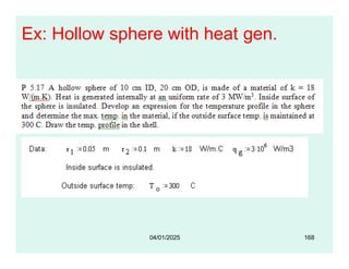
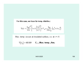
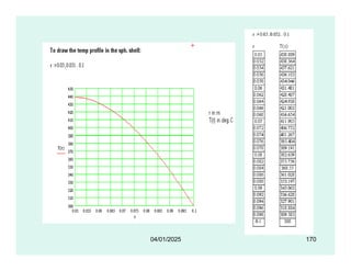
16.
Boundary and InitialConditions
Four kinds of boundary conditions
1. Dirichlet (or first-type) boundary condition :In heat transfer problems, this
condition corresponds to a given fixed surface temperature.
2. Neumann (or second-type) boundary condition :
In heat transfer problems, the Neumann condition corresponds to a given rate
of change of temperature. In other words, this condition assumes that the
heat flux at the surface of the material is known. The heat flux in the positive x-
direction anywhere in the medium, including the boundaries, can be expressed
by Fourier’s law of heat conduction.
04/01/2025 1
6
17.
Boundary and InitialConditions
Special Case – Adiabatic Boundary – Perfectly Insulated Boundary
A special case of this condition corresponds to the perfectly insulated surface for
which (∂T/∂x = 0). Heat transfer through a properly insulated surface can be
taken to be zero since adequate insulation reduces heat transfer through a
surface to negligible levels. Mathematically, this boundary condition can be
expressed as:
Special Case – Thermal Symmetry
Another very important case, that can be used for solving heat transfer problems
involving fuel rods, is the thermal symmetry. For example, the two surfaces of a
large hot plate of thickness L suspended vertically in air will be subjected to the
same thermal conditions, and thus the temperature distribution will be
symmetrical (i.e. in one half of the plate will be the same temperature profile as
that in the other half). As a result, there must be a maximum in in the center line
of the plate and the center line can be viewed as an insulated surface (∂T/∂x =
0). The thermal condition at this plane of symmetry can be expressed as:
04/01/2025 1
7
18.
1. Plane Slab
Q
T1
T2
T(x)
•Assumptions:
• One dimensional conduction i.e.
thickness L is small compared to
the dimensions in the y and z
directions
• Steady state conduction i.e.
temperature at any point within the
slab does not change with time; of
course, temperatures at different
points within the slab will be
different.
• No internal heat generation
• Material of the slab is
homogeneous (i.e. constant
density) and isotropic (i.e. value of k
is same in all directions).
X
T1 T2
slab
R = L/(kA)
L
Q
Q
Fig. 4.1 Plane slab and Thermal circuit
1
8
04/01/2025
19.
Plane Slab (contd.)
•We start with the general differential
equation in Cartesian coordinates:
1
9
04/01/2025
• So, thegoverning equation for the plane
slab with the above-mentioned
assumptions becomes:
Temperature field is obtained by solving equation (4.2):
21
04/01/2025
22.
C1 and C2are obtained from Boundary conditions:
• B.C.(i): T = T1 at x = 0
• B.C.(ii): T = T2 at x = L
• Solving:
Equation (4.4) can be written in non-dimensional form as follows:
22
04/01/2025
23.
Next, to findthe heat flux: Apply Fourier’s Law:
And,
Also, i.e.
23
04/01/2025
24.
Heat transfer throughcomposite
slabs:
T , h
b
b
Fluid flow
Fluid flow
Ta, ha
1 2 3
k1 k2 k3
Q Q
T1 T2 T3 T4
Temp. Profile
• Assumptions:
• Steady state, one
dimensional
heat conduction
• No internal heat
generation
• Constant thermal
conductivities k1, k2 and
k3
• There is ‘perfect thermal
contact’ between layers
i.e. there is no temperature
drop at the interface and
the temperature profile is
continuous
L1 L2
X
L3
Fig. 4.2 Composite slab with three layers
and the Thermal resistance network
Q
b
T1 T2 T3 T4 T
a
R R1 R2 R3 R
24
b
Ta
Q
04/01/2025
25.
• Observe thatheat flows from the fluid at
temperature Ta to the left surface of slab 1 by
convection, then by conduction through slabs 1,
2 and 3, and then, by convection from the right
surface of slab 3 to the fluid at temperature Tb.
• Now, considering each case by turn:
• Convection at the left surface of slab 1:
• Q = ha A (Ta – T1), from Newton’s Law of
cooling; i.e.
25
04/01/2025
• Conduction throughslab 3 :
Convection at the right surface of slab 3:
27
04/01/2025
28.
• Adding (a),(b) , (c) , (d) and (e):
where
28
Ra = convective resistance at left surface of slab 1,
R1 = conductive resistance of slab 1,
R2 = conductive resistance of slab 2,
R3 = conductive resistance of slab 3, and
Rb = convective resistance at right surface of slab
3
04/01/2025
29.
• So, wewrite equation (g) as:
Now, observe the analogy with Ohm’s Law.
For thermal resistances in series, we have:
29
04/01/2025
30.
• When theresistances are
in parallel, the total
resistance is given by:
Q
L
k1
k2
1
2
T1 T2
T1 T2
Q
Insulated
Q
T1 T2
X
R1=
L/(k1A)
Q
R2= L/(k2A)
Fig. 4.3 Composite slab with parallel
resistances
30
04/01/2025
31.
For thermal resistancesin series and parallel:
• Applying the rules of electrical
circuit for series and parallel
resistances, we have:
1 2
3
Q
T4
T1
T2 T3
5
Q
4
Insulation
Q Q
T1
T2 T3
T4
R1
R2
R3 R5
R4
Fig. 4.4 Composite slab with series-parallel resistances
and the equivalent Thermal circuit
Note: Conditions to be satisfied to apply this
concept are: (i) steady state heat transfer and
(ii) no internal heat generation.
31
04/01/2025
32.
Overall heat transfercoefficient, U (W/(m2.C)):
• We would like to have the heat transfer given by
a simple relation of the form:
• Q = U A (Ta – Tb) = U A T……(4.21)
• Now, we have from eqn. (4.16):
32
04/01/2025
33.
• Comparing eqn(4.16) and eqn. (4.21), we
can write:
Remember the expression for U as given by eqn. (4.23); it is easier
and is applicable when we deal with other geometries too.
33
04/01/2025
34.
Thermal contact resistance:
AB
Q
T1
Interface
T2
Air gap
A B
Q
T
• Physical reasoning for contact
resistance is explained with
reference to Fig. 4.5:
• Physical contact between A
and B occurs only at a few
points i.e. at the ‘peaks’ as
shown.
• Therefore, heat transfer
occurs by conduction through
this solid contact area and
also by ‘gas conduction’
through the
gas filling the interfacial voids.
X
X
Q
Tc1
Rcontact
R1 R2
T1 T2 Ta
Q
T1
T2
Tc1
Tc2
Tc2
Fig. 4.5 Thermal contact resistance
34
04/01/2025
35.
• In effect,resistance to heat transfer is by two
mechanisms:
• by solid conduction at the peaks, and
• by gas conduction through the interfacial gas in the
voids.
• Of these two, solid conduction is usually negligible.
• Note that that there is a temperature drop at the
interface, (Tc1 – Tc2) and the temperature profile is
not continuous.
• Thermal contact resistance is defined as the
temperature drop at the interface divided by the heat
transfer rate per unit area:
35
04/01/2025
36.
• Interface ‘thermalcontact conductance’ is defined as the
inverse of the contact resistance, and is given by:
Thermal contact resistance depends on:
•surface roughness — smoother the surface, lesser the
resistance
.interface temperature — higher the temperature, lesser the
resistance
•interface pressure — higher the pressure, lesser the resistance
•type of material – softer the material, lesser the resistance
36
04/01/2025
37.
• Thermal contactresistance may be reduced
by:
• making the mating surfaces very smooth
• inserting a layer of conducting grease at the
interface
• inserting a ‘shim’ (thin foil) made of a soft material
such as indium, lead, tin or silver between the
surfaces
• filling the interstitial voids with a gas of higher thermal
conductivity than that of air (ex: helium)
• increasing the interface pressure
• in case of permanently bonded joints, contact
resistance can be reduced by using an epoxy or soft
solder rich in lead, or a hard solder of gold/tin alloy
• Values of Rc are given in Heat Transfer Handbooks.
37
04/01/2025
Cylindrical systems (contd.)
•Assumptions:
• Steady state conduction
• One dimensional conduction, in the r-
direction only
• Homogeneous, isotropic material with
constant k
• No internal heat generation
41
04/01/2025
42.
Cylindrical systems (contd.)
•In cylindrical coordinates, we have the general diff.
eqn. for conduction:
In this case:
42
04/01/2025
43.
Cylindrical systems (contd.)
•Therefore, the controlling differential equation for the
cylindrical system becomes:
Integrating above eqn. twice:
43
04/01/2025
44.
• C1 andC2 are found out by applying the two
B.C’s: at r = ri, T = Ti
at r = ro, T
= To Solving, we
get:
Eqn. (4.34) is written in non-dimensional form as follows:
Note: For thin cylinders, ri ro , and then the temperature
distribution within the shell is almost linear.
44
04/01/2025
45.
• Next, tofind the heat transfer rate, Q:
• We apply the Fourier’s Law.
• Considering the inner radius ri,
Equation (4.36) gives the desired expression for rate of heat
transfer through the cylindrical system.
45
04/01/2025
46.
Thermal resistance ofcyl. system
• Now, writing eqn. (4.36) in a form analogous to Ohm’s
Law:
Therefore,
46
04/01/2025
Composite cylinders (contd.):
•Assumptions:
• Steady state heat flow
• One dimensional conduction in the r direction only
• No internal heat generation
• Perfect thermal contact between layers
• Under these stipulations, we note that heat flow rate is
constant and the same through each layer.
• Let us write separately the heat flow equations for
each layer:
48
04/01/2025
49.
• 1. Convectionfrom the hot fluid to inner wall at T1:
2. Conduction through first cylindrical layer:
49
04/01/2025
50.
• 3. Conductionthrough second cylindrical layer:
4. Convection from the outer wall at T3 to cold fluid at Tb:
50
04/01/2025
51.
• Adding equations(a), (b), (c) and (d):
(Ta – Tb) = Q (Ra + R1 + R2 + Rb)
If there are N concentric cylinders, we can write :
51
04/01/2025
52.
Overall heat transfercoefficient for the
cylindrical system:
• We would like to write the heat transfer rate in terms of
the known overall temperature difference, as follows:
Q = U A Toverall = U A (Ta – Tb)
where U is an overall heat transfer coefficient and A is
the area normal to the direction of heat flow.
• In the case of a cylindrical system, area normal to the
direction of heat flow is 2rL, and clearly, this varies
with
r. Therefore, while dealing with cylindrical systems, we
have to specify as to which area U is based on i.e.
whether it is based on inside area or outside area.
52
04/01/2025
Spherical Systems (contd.):
•Assumptions:
• Steady state conduction
• One dimensional conduction, in the r direction only
• Homogeneous, isotropic material with constant k
• No internal heat generation
For one dimensional conduction in r - direction
only, we have:
57
04/01/2025
58.
• For theabove mentioned assumptions, this reduces to:
i.e.
Integrating:
58
04/01/2025
59.
• Integrating again,
whereC1 and C2 are constants of integration, found
out by applying the two B.C’s, viz.:
at r = ri, T = Ti
at r = ro, T =
To
Getting and
substituting C1
and C2 in eqn.
(4.51), we
have:
59
04/01/2025
60.
• Eqn. (4.52)is written in non-dimensional form as follows:
Next, to find the heat transfer rate, Q:
We apply the Fourier’s Law. Since it is steady state conduction, with
no heat generation, Q is the same through each layer.
Considering the outer surface, i.e. at r = ro:
60
04/01/2025
61.
Thermal resistance for
conductionfor a spherical shell:
• Now, writing eqn. (4.54) in a form analogous to Ohm’s
Law:
Then, thermal resistance for conduction for a spherical shell is given by:
61
04/01/2025
Composite Spheres:
• Assumptions:
•Steady state heat flow
• One dimensional conduction in the r direction only
• No internal heat generation
• Perfect thermal contact between layers
• Under the given stipulations, it is clear that heat flow
rate, Q through each layer is the same.
• Let us write separately the heat flow equations for
each layer:
63
04/01/2025
64.
• 1. Convectionfrom the hot fluid to inner wall at T1:
2. Conduction through first spherical layer:
64
04/01/2025
65.
• 3. Conductionthrough second spherical layer:
4. Convection from the outer wall at T3 to cold fluid at T :
65
04/01/2025
66.
• Adding equations(a), (b), (c) and (d):
(Ta – Tb) = Q (Ra + R1 + R2 + Rb)
If there are N concentric spheres, we can
write :
66
04/01/2025
67.
Overall heat transfercoefficient for
the spherical system:
• We write:
67
04/01/2025
68.
Overall heat transfercoefficient for
the spherical system (contd.):
• We can also write:
And,
68
04/01/2025
69.
Overall heat transfercoefficient for
the spherical system (contd.):
• Note: Equations (4.62 a) and (4.62 b) give Ui and Uo in
terms of the inside and outside radii.
• You need not memorize them.
• To calculate Ui or Uo while solving numerical
problems, just remember equation (4.46), viz.:
69
04/01/2025
70.
4. Critical thicknessof insulation
for cylindrical system:
• Generally, addition of insulation
does reduce the heat loss.
• However, there are some
interesting cases where the
increases the heat loss!
• Consider a cylinder with
insulation where r1 is the
inner radius of insulation layer
(or, outer radius of pipe), r2 is
the outer radius of insulation
layer. 70
04/01/2025
71.
Critical thickness of
insulation(contd.):
•Resistance to heat transfer is made up of two
components viz. conductive resistance through
the cylindrical insulation layer [ R= ln(r2/r1)/ (2 k
L) ] and convective resistance between the wall
surface and the surroundings [Ro = 1/(h. Ao )].
• As the insulation thickness is increased i.e. as
insulation radius r2 is increased, conductive
resistance of insulation increases; however,
convective resistance, given by [Ro =1/(h. Ao)]
goes on decreasing since Ao, the outside
surface area goes on increasing with
increasing radius.
71
04/01/2025
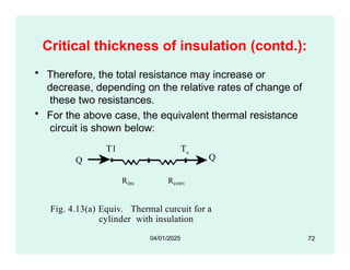
72.
Critical thickness ofinsulation (contd.):
• Therefore, the total resistance may increase or
decrease, depending on the relative rates of change of
these two resistances.
• For the above case, the equivalent thermal resistance
circuit is shown below:
T1 Ta
Q
Q
Rins Rconv
Fig. 4.13(a) Equiv. Thermal curcuit for a
cylinder with insulation
72
04/01/2025
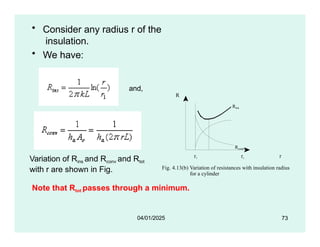
73.
• Consider anyradius r of the
insulation.
• We have:
and,
R
Rtot
Rins
Variation of Rins and Rconv and Rtot
with r are shown in Fig.
Rconv
73
r1 rc r
Fig. 4.13(b) Variation of resistances with insulation radius
for a cylinder
Note that Rtot passes through a minimum.
04/01/2025
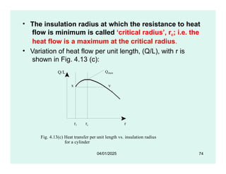
74.
• The insulationradius at which the resistance to heat
flow is minimum is called ‘critical radius’, rc; i.e. the
heat flow is a maximum at the critical radius.
• Variation of heat flow per unit length, (Q/L), with r is
shown in Fig. 4.13 (c):
Q/L Qmax
y
x
r1 rc r
Fig. 4.13(c) Heat transfer per unit length vs. insulation radius
for a cylinder
74
04/01/2025
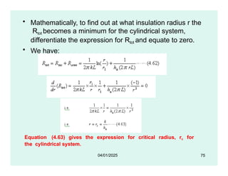
75.
• Mathematically, tofind out at what insulation radius r the
Rtot becomes a minimum for the cylindrical system,
differentiate the expression for Rtot and equate to zero.
• We have:
Equation (4.63) gives the expression for critical radius, rc for
the cylindrical system.
75
04/01/2025
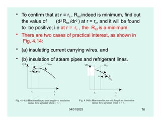
76.
• To confirmthat at r = rc , Rtot indeed is minimum, find out
the value of (d2 Rtot /dr2 ) at r = rc, and it will be found
to be positive; i.e at r = rc , the Rtot is a minimum.
• There are two cases of practical interest, as shown in
Fig. 4.14:
• (a) insulating current carrying wires, and
• (b) insulation of steam pipes and refrigerant lines.
r1 rc
r
Fig. 4.14(a) Heat transfer per unit length vs. insulation
radius for a cylinder when r1 < r c
Q/L Qmax
a b
Q/L Qmax
a b
rc r1
r
Fig. 4.14(b) Heat transfer per unit length vs. insulation
radius for a cylinder when r1 > r c
76
04/01/2025
77.
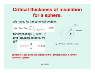
Critical thickness ofinsulation
for a sphere:
r1
r
Insulation
• We have, for the spherical system:
Sphere
Fig. 4.15 Critical radius for a Sphere
Differentiating Rtot w.r.t. r
and equating to zero, we
get:
Equation (4.66) gives the expression for critical radius, rc for the
spherical system.
77
04/01/2025
78.
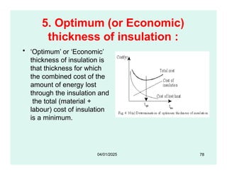
5. Optimum (orEconomic)
thickness of insulation :
• ‘Optimum’ or ‘Economic’
thickness of insulation is
that thickness for which
the combined cost of the
amount of energy lost
through the insulation and
the total (material +
labour) cost of insulation
is a minimum.
78
04/01/2025
79.
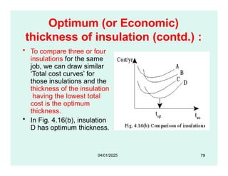
Optimum (or Economic)
thicknessof insulation (contd.) :
• To compare three or four
insulations for the same
job, we can draw similar
‘Total cost curves’ for
those insulations and the
thickness of the insulation
having the lowest total
cost is the optimum
thickness.
• In Fig. 4.16(b), insulation
D has optimum thickness.
79
04/01/2025
80.
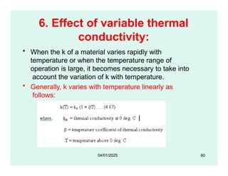
6. Effect ofvariable thermal
conductivity:
• When the k of a material varies rapidly with
temperature or when the temperature range of
operation is large, it becomes necessary to take into
account the variation of k with temperature.
• Generally, k varies with temperature linearly as
follows:
80
04/01/2025
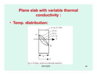
81.
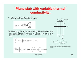
Plane slab withvariable thermal
conductivity:
• We write from Fourier’s Law:
k = k(T)
Q
T1 T2
X
dX
Substituting for k(T), separating the variables and
integrating from x = 0 to x = L (with T = T1 to T =
T2):
X
T1 T2
L
Q
Q
Rslab = L/(kmA)
Fig. 4.17 Plane slab with k = k(T) and the thermal
circuit
81
04/01/2025
82.
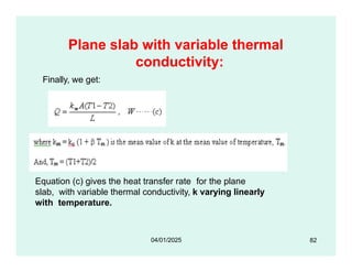
Plane slab withvariable thermal
conductivity:
Finally, we get:
Equation (c) gives the heat transfer rate for the plane
slab, with variable thermal conductivity, k varying linearly
with temperature.
82
04/01/2025
83.
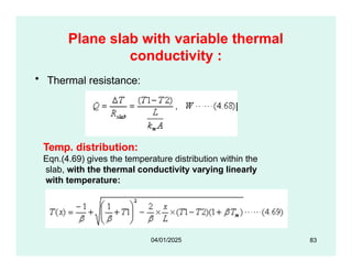
Plane slab withvariable thermal
conductivity :
• Thermal resistance:
Temp. distribution:
Eqn.(4.69) gives the temperature distribution within the
slab, with the thermal conductivity varying linearly
with temperature:
83
04/01/2025
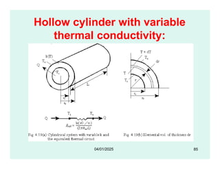
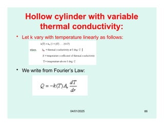
Hollow cylinder withvariable
thermal conductivity:
• Let k vary with temperature linearly as follows:
• We write from Fourier’s Law:
86
04/01/2025
87.
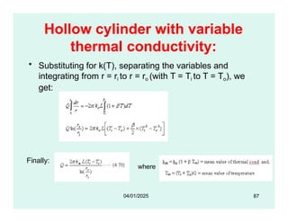
Hollow cylinder withvariable
thermal conductivity:
• Substituting for k(T), separating the variables and
integrating from r = ri to r = ro (with T = Ti to T = To), we
get:
Finally:
where
87
04/01/2025
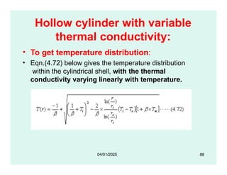
88.
Hollow cylinder withvariable
thermal conductivity:
• To get temperature distribution:
• Eqn.(4.72) below gives the temperature distribution
within the cylindrical shell, with the thermal
conductivity varying linearly with temperature.
88
04/01/2025
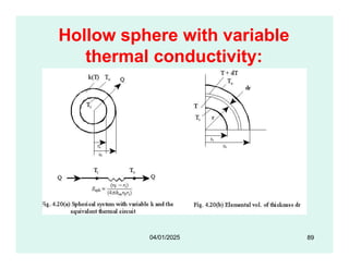
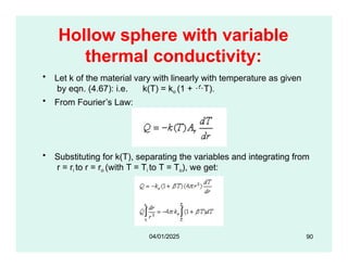
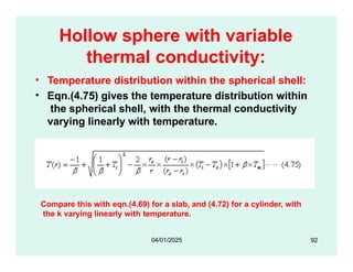
Hollow sphere withvariable
thermal conductivity:
• Let k of the material vary with linearly with temperature as given
by eqn. (4.67): i.e. k(T) = ko (1 + T).
• From Fourier’s Law:
• Substituting for k(T), separating the variables and integrating from
r = ri to r = ro (with T = Ti to T = To), we get:
90
04/01/2025
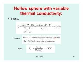
Hollow sphere withvariable
thermal conductivity:
• Temperature distribution within the spherical shell:
• Eqn.(4.75) gives the temperature distribution within
the spherical shell, with the thermal conductivity
varying linearly with temperature.
Compare this with eqn.(4.69) for a slab, and (4.72) for a cylinder, with
the k varying linearly with temperature.
92
04/01/2025
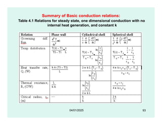
93.
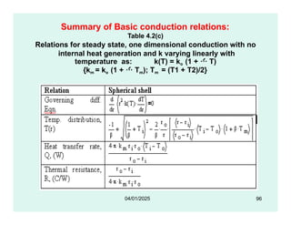
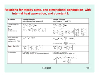
Summary of Basicconduction relations:
Table 4.1 Relations for steady state, one dimensional conduction with no
internal heat generation, and constant k
93
04/01/2025
94.
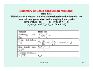
Summary of Basicconduction relations:
Table 4.2(a)
Relations for steady state, one dimensional conduction with no
internal heat generation and k varying linearly with
temperature as: k(T) = ko (1 + T)
{km = ko (1 + Tm); Tm = (T1 + T2)/2}
94
04/01/2025
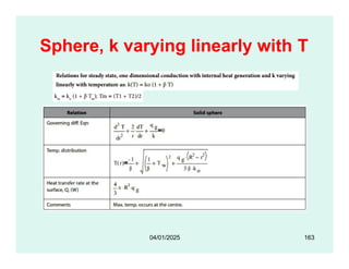
95.
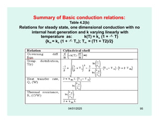
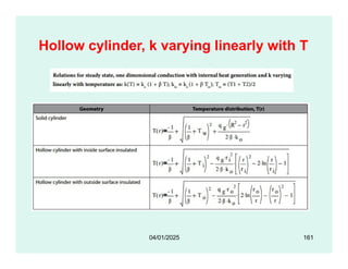
Summary of Basicconduction relations:
Table 4.2(b)
Relations for steady state, one dimensional conduction with no
internal heat generation and k varying linearly with
temperature as: k(T) = ko (1 + T)
{km = ko (1 + Tm); Tm = (T1 + T2)/2}
95
04/01/2025
96.
Summary of Basicconduction relations:
Table 4.2(c)
Relations for steady state, one dimensional conduction with no
internal heat generation and k varying linearly with
temperature as: k(T) = ko (1 + T)
{km = ko (1 + Tm); Tm = (T1 + T2)/2}
96
04/01/2025
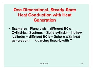
97.
One-Dimensional, Steady-State
Heat Conductionwith Heat
Generation
• Examples - Plane slab – different BC’s -
Cylindrical Systems – Solid cylinder – hollow
cylinder – different BC’s – Sphere with heat
generation- k varying linearly with T
04/01/2025 97
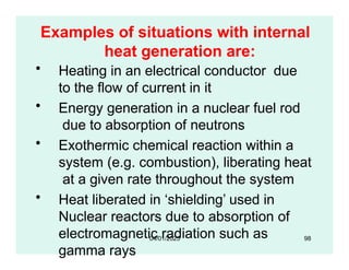
98.
Examples of situationswith internal
heat generation are:
• Heating in an electrical conductor due
to the flow of current in it
• Energy generation in a nuclear fuel rod
due to absorption of neutrons
• Exothermic chemical reaction within a
system (e.g. combustion), liberating heat
at a given rate throughout the system
• Heat liberated in ‘shielding’ used in
Nuclear reactors due to absorption of
electromagnetic radiation such as
gamma rays
04/01/2025 98
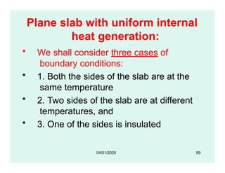
99.
Plane slab withuniform internal
heat generation:
• We shall consider three cases of
boundary conditions:
• 1. Both the sides of the slab are at the
same temperature
• 2. Two sides of the slab are at different
temperatures, and
• 3. One of the sides is insulated
04/01/2025 99
100.
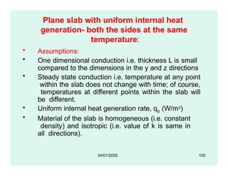
Plane slab withuniform internal heat
generation- both the sides at the same
temperature:
• Assumptions:
• One dimensional conduction i.e. thickness L is small
compared to the dimensions in the y and z directions
• Steady state conduction i.e. temperature at any point
within the slab does not change with time; of course,
temperatures at different points within the slab will
be different.
• Uniform internal heat generation rate, qg (W/m3)
• Material of the slab is homogeneous (i.e. constant
density) and isotropic (i.e. value of k is same in
all directions).
04/01/2025 100
101.
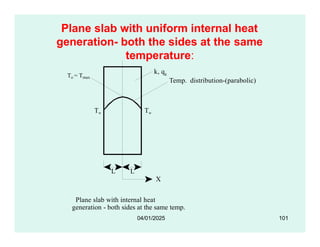
Plane slab withuniform internal heat
generation- both the sides at the same
temperature:
k, qg
Tw
To = Tmax
Tw
Temp. distribution-(parabolic)
X
Plane slab with internal heat
generation - both sides at the same temp.
L
L
04/01/2025 101
102.
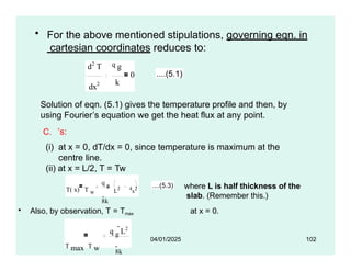
• For theabove mentioned stipulations, governing eqn. in
cartesian coordinates reduces to:
dx2 k
d2
T q g
0 ....(5.1)
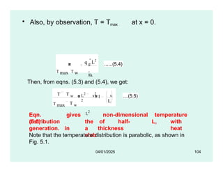
• Also, by observation, T = Tmax at x = 0.
Solution of eqn. (5.1) gives the temperature profile and then, by
using Fourier’s equation we get the heat flux at any point.
C. ’s:
(i) at x = 0, dT/dx = 0, since temperature is maximum at the
centre line.
(ii) at x = L/2, T = Tw
04/01/2025 102
T( x) T w
q g
8k
L2 4
x2 ....(5.3) where L is half thickness of the
slab. (Remember this.)
q g
L2
T max T w 8k
• Also, byobservation, T = Tmax at x = 0.
q g
L2
T max T w 8k
......(5.4)
Then, from eqns. (5.3) and (5.4), we get:
T T w
T max T w
1
L
L
2
x
2
x
2
L
2
....(5.5)
04/01/2025 104
Eqn.
(5.5)
distribution
gives
the
in a
slab
non-dimensional
of half-
thickness
temperature
L, with
heat
generation.
Note that the temperature distribution is parabolic, as shown in
Fig. 5.1.
105.
Convection boundary condition:
•In many practical applications, heat is carried
away at the boundaries by a fluid at a
temperature Tf flowing on the surface with a
convective heat transfer coefficient, h. (e.g.
current carrying conductor cooled by ambient air
or nuclear fuel rod cooled by a liquid metal
coolant).
• Then, by an energy balance at the surface:
• heat conducted from within the body to the
surface = the heat convected away by the
fluid at the surface.
04/01/2025 105
106.
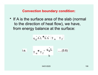
Convection boundary condition:
•If A is the surface area of the slab (normal
to the direction of heat flow), we have,
from energy balance at the surface:
q g
A L h A T w T f
i.e.
T w T f
q g
L
h
.....(5.6)
04/01/2025 106
107.
• Substituting eqn.(5.6) in eqn.
(5.3),
h 2k
T( x) T f
L
x
2 2
q g
L q g ......(5.7)
Eqn. (5.7) gives temperature distribution in a slab with heat
generation, in terms of the fluid temperature, Tf .
Remember, again, that L is half-thickness of the slab.
Heat transfer:
By observation, we know that the heat transfer rate from
either of the surfaces must be equal to half of the total
heat generated within the slab, for the B.C. of Tw being
the same at both the surfaces.
i.e. Q = qg A L……..(5.8)
04/01/2025 107
108.
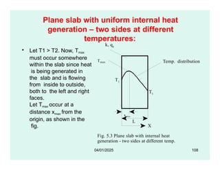
Plane slab withuniform internal heat
generation – two sides at different
temperatures:
k, qg
• Let T1 > T2. Now, Tmax
Tmax
T1
Temp. distribution
must occur somewhere
within the slab since heat
is being generated in
the slab and is flowing
from inside to outside,
both to the left and right
faces.
Let Tmax occur at a
distance xmax from the
origin, as shown in the
fig. X
Fig. 5.3 Plane slab with internal heat
generation - two sides at different temp.
T2
L
xmax
04/01/2025 108
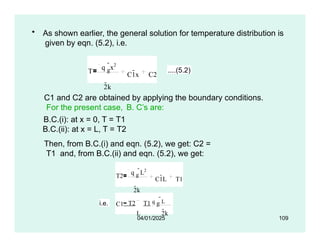
109.
• As shownearlier, the general solution for temperature distribution is
given by eqn. (5.2), i.e.
T
q g
x2
2k
C1x C2
....(5.2)
C1 and C2 are obtained by applying the boundary conditions.
For the present case, B. C’s are:
B.C.(i): at x = 0, T = T1
B.C.(ii): at x = L, T = T2
Then, from B.C.(i) and eqn. (5.2), we get: C2 =
T1 and, from B.C.(ii) and eqn. (5.2), we get:
T2
q g
L2
2k
C1L T1
i.e. C1 T2 T1 q g
L
L 2k
04/01/2025 109
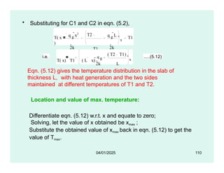
110.
• Substituting forC1 and C2 in eqn. (5.2),
T( x
)
q g
x2
2k
T2
T1
L
q g
L
2k
x
T1
i.e.
T( x) T1 ( L x)
q g
( T2 T1)
2k L
x
.....(5.12)
Eqn. (5.12) gives the temperature distribution in the slab of
thickness L, with heat generation and the two sides
maintained at different temperatures of T1 and T2.
Location and value of max. temperature:
Differentiate eqn. (5.12) w.r.t. x and equate to zero;
Solving, let the value of x obtained be xmax ;
Substitute the obtained value of xmax back in eqn. (5.12) to get the
value of Tmax.
04/01/2025 110
111.
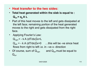
• Heat transferto the two sides:
• Total heat generated within the slab is equal to :
Qtot = qg A L
• Part of this heat moves to the left and gets dissipated at
the left face; remaining portion of the heat generated
moves to the right and gets dissipated from the right
face.
• Applying Fourier’s Law:
Qright = - k A (dT/dx)x=L
Qleft = - k A (dT/dx)x=0 …this will be -ve since heat
flows from right to left i.e. in –ve x- direction
• Of course, sum of Qright and Qleft must be equal to
Qtot.
04/01/2025 111
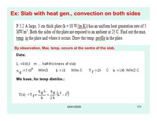
112.
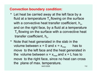
Convection boundary condition:
•Let heat be carried away at the left face by a
fluid at a temperature Ta flowing on the surface
with a convective heat transfer coefficient, ha,
and on the right face, by a fluid at a temperature
Tb flowing on the surface with a convective heat
transfer coefficient, hb.
• Note that heat generated in the slab in the
volume between x = 0 and x = xmax has to
move to the left face and the heat generated in
the volume between x = xmax and x = L has to
move to the right face, since no heat can cross
the plane of max. temperature.
04/01/2025 112
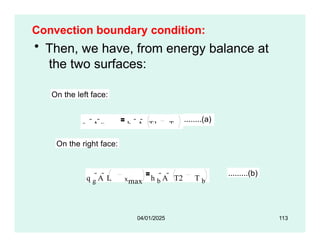
113.
Convection boundary condition:
•Then, we have, from energy balance at
the two surfaces:
On the left face:
q g
A xmax h a
A T1 T a
........(a)
On the right face:
xmax
q g
A L h b
A T2 T b
.........(b)
04/01/2025 113
114.
• From eqns.(a)and (b), we get T1
and T2 in terms of known fluid
temperatures Ta and Tb respectively.
• After thus obtaining T1 and T2,
substitute them in eqn. (5.12) to get
the temperature distribution in terms of
fluid temperatures Ta and Tb .
04/01/2025 114
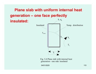
115.
Plane slab withuniform internal heat
generation – one face perfectly
insulated:
Tmax
k, qg
Insulated Temp. distribution
Tw
L
X
Fig. 5.4 Plane slab with internal heat
generation - one side insulated
ha
Ta
04/01/2025 115
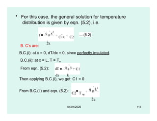
116.
• For thiscase, the general solution for temperature
distribution is given by eqn. (5.2), i.e.
T
q g
x2
2k
C1x C2
....(5.2)
B. C’s are:
B.C.(i): at x = 0, dT/dx = 0, since perfectly insulated.
B.C.(ii): at x = L, T = Tw
From eqn. (5.2): dT q g
x
dx k
C1
Then applying B.C.(i), we get: C1 = 0
From B.C.(ii) and eqn. (5.2):
C2 T w
q g
L2
2k
04/01/2025 116
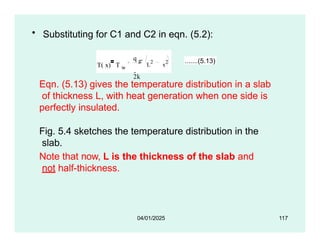
117.
• Substituting forC1 and C2 in eqn. (5.2):
T( x) T w
q g
2k
L
2
x
2 .......(5.13)
Eqn. (5.13) gives the temperature distribution in a slab
of thickness L, with heat generation when one side is
perfectly insulated.
Fig. 5.4 sketches the temperature distribution in the
slab.
Note that now, L is the thickness of the slab and
not half-thickness.
04/01/2025 117
118.
In case ofconvection boundary
condition:
• Since the left face is insulated, all the heat generated in
the slab travels to the surface on the right and gets
convected away to the fluid.
• Heat generated in the slab:
Q gen q g
A L
Heat convected at surface: Q conv h a
A T w T a
T w T a
Equating the heat generated and heat convected, we get:
q g
L
h a
....(a)
04/01/2025 118
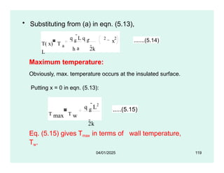
119.
• Substituting from(a) in eqn. (5.13),
a
h 2k
T( x) T a
L
x
2 2
q g
L q g .......(5.14)
Maximum temperature:
Obviously, max. temperature occurs at the insulated surface.
Putting x = 0 in eqn. (5.13):
T max T w
q g
L2
2k
.....(5.15)
04/01/2025 119
Eq. (5.15) gives Tmax in terms of wall temperature,
Tw.
120.
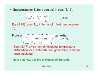
• Substituting forTw from eqn. (a) in eqn. (5.15):
T max T a
q g
L
h a
q g
L2
2k
.....(5.16)
Eq. (5.16) gives Tmax in terms of fluid temperature,
Ta.
From eqn. (5.13) and (5.15), we can write:
T( x) T w
T max T w L
2
1
L
2
x
2
x
2
L
....(5.17)
04/01/2025 120
Eqn. (5.17) gives non-dimensional temperature
distribution for a slab with heat generation, and one
face insulated.
Note that now L is the thickness of the slab.
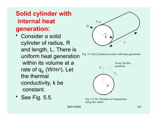
121.
Solid cylinder with
internalheat
generation:
Q
Ti
To
k, qg
Fig. 5.5 (a) Cylindrical system with heat generation
L
L
R
• Consider a solid
cylinder of radius, R
and length, L. There is
uniform heat generation
within its volume at a
rate of q (W/m3). Let
g
the thermal
conductivity, k be
constant.
• See Fig. 5.5.
Temp. Profile,
parabolic
To
Fig. 5.5 (b) Variation of temperature
along the radius
R
Tw
04/01/2025 121
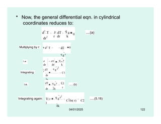
122.
• Now, thegeneral differential eqn. in cylindrical
coordinates reduces to:
dr2
d2
T 1 dT
r dr k
q g
0 ....(a)
Multiplying by r: r d2
T dT
q g
r
dr
2
dr
k
0
i.e. d dT q g
r
Integrating:
dr dr k
2
r dT q g r
dr
2k
C1
i.e.
dT q g
r
dr 2k
C1
r
......(b)
Integrating again: T( r
)
q g
r2
4k
C1ln( r) C2
.....(5.18)
04/01/2025 122
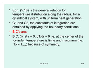
123.
• Eqn. (5.18)is the general relation for
temperature distribution along the radius, for a
cylindrical system, with uniform heat generation.
• C1 and C2, the constants of integration are
obtained by applying the boundary conditions.
• B.C’s are:
• B.C. (i): at r = 0, dT/dr = 0 i.e. at the center of the
cylinder, temperature is finite and maximum (i.e.
To = Tmax) because of symmetry.
04/01/2025 123
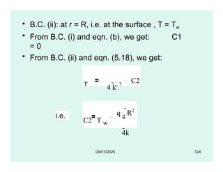
124.
T w
• B.C.(ii): at r = R, i.e. at the surface , T = Tw
• From B.C. (i) and eqn. (b), we get: C1
= 0
• From B.C. (ii) and eqn. (5.18), we get:
q g
R
2
C2
4 k
i.e.
C2 T w
q g
R2
4k
04/01/2025 124
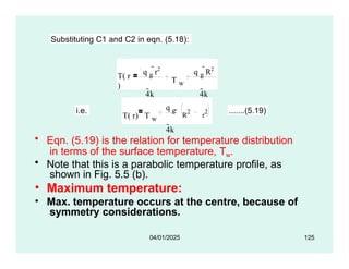
125.
Substituting C1 andC2 in eqn. (5.18):
T( r
)
q g
r2
4k
T w
q g
R2
4k
i.e.
T( r) T w
q g
4k
R
2
r
2 .......(5.19)
• Eqn. (5.19) is the relation for temperature distribution
in terms of the surface temperature, Tw.
• Note that this is a parabolic temperature profile, as
shown in Fig. 5.5 (b).
• Maximum temperature:
• Max. temperature occurs at the centre, because of
symmetry considerations.
04/01/2025 125
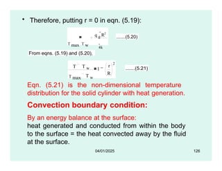
126.
• Therefore, puttingr = 0 in eqn. (5.19):
q g
R2
T max T w 4k
.......(5.20)
From eqns. (5.19) and (5.20),
T T w
T max T w
1
r
R
2
.......(5.21)
Eqn. (5.21) is the non-dimensional temperature
distribution for the solid cylinder with heat generation.
Convection boundary condition:
By an energy balance at the surface:
heat generated and conducted from within the body
to the surface = the heat convected away by the fluid
at the surface.
04/01/2025 126
127.
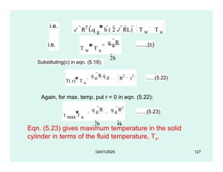
i.e.
R2 Lqg h ( 2 RL) T w T a
i.e.
T w T a
q g
R
2h
.......(c)
Substituting(c) in eqn. (5.19):
T( r) T a
R r
2 2
q g
R q g
2h 4k
......(5.22)
Again, for max. temp. put r = 0 in eqn. (5.22):
T max T a
q g
R q g
R2
2h 4k
.......(5.23)
04/01/2025 127
Eqn. (5.23) gives maximum temperature in the solid
cylinder in terms of the fluid temperature, Ta.
128.
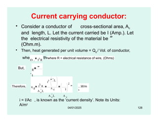
Current carrying conductor:
•Consider a conductor of cross-sectional area, Ac
and length, L. Let the current carried be I (Amp.). Let
the electrical resistivity of the material be
(Ohm.m).
• Then, heat generated per unit volume = Qg / Vol. of conductor,
where Qg is the total heat generated (W).
Q g I2 R
where R = electrical resistance of wire, (Ohms)
But, R
L
A c
Therefore, q g
2
R
I
A c
L
I
2 L
A c I
A c
L A c
2
04/01/2025 128
...W/m
3
i = I/Ac , is known as the ‘current density’. Note its Units:
A/m2
129.
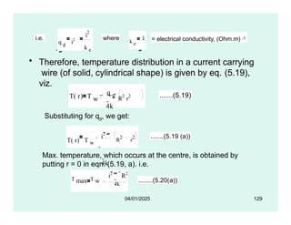
• Therefore, temperaturedistribution in a current carrying
wire (of solid, cylindrical shape) is given by eq. (5.19),
viz.
i.e.
q g i2
i
2
k e
where k e
1
= electrical conductivity, (Ohm.m) -1
T( r) T w
4k
q g R
2
r
2 .......(5.19)
Substituting for qg, we get:
T( r) T w R
2
r
2
i2
4k
.......(5.19 (a))
Max. temperature, which occurs at the centre, is obtained by
putting r = 0 in eqn. (5.19, a). i.e.
i2 R2
T max T w 4k
........(5.20(a))
04/01/2025 129
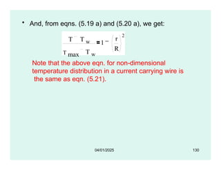
130.
• And, fromeqns. (5.19 a) and (5.20 a), we get:
T T w
T max T w
1
r
R
2
Note that the above eqn. for non-dimensional
temperature distribution in a current carrying wire is
the same as eqn. (5.21).
04/01/2025 130
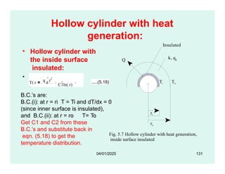
131.
Hollow cylinder withheat
generation:
the inside surface
insulated:
• We have:
k, qg
Q
To Ti To
Insulated
• Hollow cylinder with
T( r
)
q g
r2
4k
C1ln( r)
C2
.....(5.18)
Fig. 5.7 Hollow cylinder with heat generation,
inside surface insulated
ri
ro
B.C.’s are:
B.C.(i): at r = ri T = Ti and dT/dx = 0
(since inner surface is insulated),
and B.C.(ii): at r = ro T= To
Get C1 and C2 from these
04/01/2025 131
B.C.’s and substitute back in
eqn. (5.18) to get the
temperature distribution.
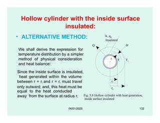
132.
Hollow cylinder withthe inside surface
insulated:
• ALTERNATIVE METHOD:
Q
Ti To
k, qg
Insulated
dr
r
Fig. 5.8 Hollow cylinder with heat generation,
inside surface insulated
ri
ro
equal to the heat conducted
away from the surface at radius r.
04/01/2025 132
We shall derive the expression for
temperature distribution by a simpler
method of physical consideration
and heat balance:
Since the inside surface is insulated,
heat generated within the volume
between r = ri and r = r, must travel
only outward; and, this heat must be
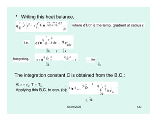
133.
• Writing thisheat balance,
g
q r r i
2 2
L k2 rL dT
dr
where dT/dr is the temp. gradient at radius r.
i.e. dT
q r
2
g i dr q g
2k r 2k
rdr
Integrating, T( r
)
q gr
2
i ln( r)
q gr
2
C .....(b)
2k 4k
The integration constant C is obtained from the B.C.:
At r = ro, T = To
Applying this B.C. to eqn. (b):
q
C T o
2
r
q
g
o 4k
r
2
2k
g i ln r o
04/01/2025 133
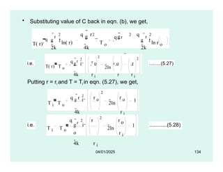
134.
• Substituting valueof C back in eqn. (b), we get,
T( r)
q
2k
g i ln( r)
g
q r
4k
T o
q r
q
g
o 4k
r
2 2 2 r
2
2k
g i ln r o
i.e.
T( r) T o
q r 2
2
2ln
r
2
g i
r o o r
4k r i r r i
.........(5.27)
Putting r = ri and T = Ti in eqn. (5.27), we get,
T i T o
q g
r 2
r o
4k
r i
2
r o
r i
2ln 1
i
i.e.
T i T o
q r
2 r
2
r o
r i
2ln
1
g i
o
4k r i
............(5.28)
04/01/2025 134
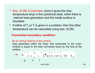
135.
• Eqn. (5.28)is important, since it gives the max.
temperature drop in the cylindrical shell, when there is
internal heat generation and the inside surface is
insulated.
• If either of To or Ti is given in a problem, then the other
temperature can be calculated using eqn. (5.28).
Convection boundary condition:
By an energy balance at the surface:
heat generated within the body and conducted to the outer
surface is equal to the heat convected away by the fluid at the
surface.
i.e. q
2
2
g o i
a o o
r r L h 2 r L T T a
04/01/2025 135
136.
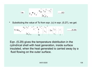
• Substituting thevalue of To from eqn. (c) in eqn. (5.27), we get:
i.e.
T o T a
q r r
g o i
2 2
2h a
r o
......(c)
T( r) T a
q g
r o
2
r 2
i
2h a
r o
q r 2
g
i
4k
r o
2
r i
2ln
r o
r i
r
2
r i
.........(5.29)
Eqn. (5.29) gives the temperature distribution in the
cylindrical shell with heat generation, inside surface
insulated, when the heat generated is carried away by a
fluid flowing on the outer surface.
04/01/2025 136
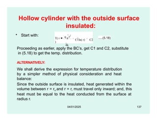
137.
Hollow cylinder withthe outside surface
insulated:
• Start with:
T( r
)
q g
r2
4k
C1ln( r) C2
.....(5.18)
Proceeding as earlier, apply the BC’s, get C1 and C2, substitute
in (5.18) to get the temp. distribution.
ALTERNATIVELY:
We shall derive the expression for temperature distribution
by a simpler method of physical consideration and heat
balance:
Since the outside surface is insulated, heat generated within the
volume between r = ro and r = r, must travel only inward; and, this
heat must be equal to the heat conducted from the surface at
radius r.
04/01/2025 137
138.
• Writing thisheat balance,
Q
Ti Insulate
d dr
k, qg
To
Note that the term on the
RHS has +ve sign,
since, now, the heat
transfer is from
Fig. 5.10 Hollow cylinder with heat generation,
outside surface insulated
ri
ro
outside to inside, i.e. in the
–ve r-direction (because
the outside surface is
insulated).
04/01/2025 138
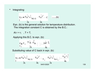
139.
• Integrating:
T( r
)
qg
r o
2
2k
ln( r)
q g
r2
4k
C .......(b)
Eqn. (b) is the general solution for temperature distribution.
The integration constant C is obtained by the B.C.:
At r = ri , T = Ti
Applying this B.C. to eqn. (b):
2
r
2k
q
C T i
g o ln
r i
q r
2
g i
4k
Substituting value of C back in eqn. (b):
T( r
)
q g
r o
2
2k
ln( r)
q g
r2
4k
T i
q g
r o
2
2k
ln r i
q r
2
g i
4k
04/01/2025 139
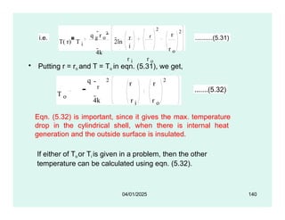
140.
• Putting r= ro and T = To in eqn. (5.31), we get,
i.e.
T( r) T i
q g
r o
2
4k
2ln
r r
i
r i r o
2
r
r o
2
..........(5.31)
T o
r
r r
2 2
q
4k r i r o
.......(5.32)
Eqn. (5.32) is important, since it gives the max. temperature
drop in the cylindrical shell, when there is internal heat
generation and the outside surface is insulated.
If either of Toor Ti is given in a problem, then the other
temperature can be calculated using eqn. (5.32).
04/01/2025 140
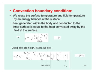
141.
• Convection boundarycondition:
• We relate the surface temperature and fluid temperature
by an energy balance at the surface:
• heat generated within the body and conducted to the
inner surface is equal to the heat convected away by the
fluid at the surface.
q r
2 2
r
i.e. T i T a
g o i ......(c)
2h a
r i
Using eqn. (c) in eqn. (5.31), we get:
T( r) T a
q g
r o
2
r 2
i
2h a
r i
q
g
r o
2
4k
2ln
r
r i
r i
r o
2
r
2
r o
.......(5.33)
04/01/2025 141
142.
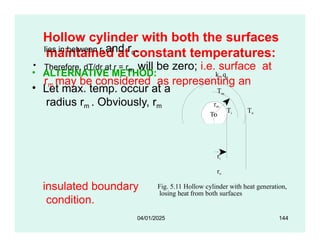
Hollow cylinder withboth the surfaces
maintained at constant
temperatures:
• We have for temp.
distribution:
i
T To
rm
To
k, qg
Tm
T( r
)
q g
r2
4k
C1ln( r)
C2
.....(5.18)
Fig. 5.11 Hollow cylinder with heat generation,
losing heat from both surfaces
ri
ro
C1 and C2, the constants of
integration are obtained by
applying the boundary
conditions.
04/01/2025 142
143.
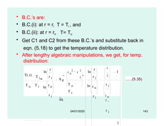
T = Ti, and
T= To
• B.C.’s are:
• B.C.(i): at r = ri
• B.C.(ii): at r = ro
• Get C1 and C2 from these B.C.’s and substitute back in
eqn. (5.18) to get the temperature distribution.
• After lengthy algebraic manipulations, we get, for temp.
distribution:
T( r) T i
ln
r
r i q g
4k
r o
2
r
2
i
T o
T i
ln
ln
r
r i
r o
r i
r
2
r i
r o
2
r i
1
T o T i ln
r o
r i
1
04/01/2025 143
......(5.35)
144.
Hollow cylinder withboth the surfaces
maintained at constant temperatures:
• ALTERNATIVE METHOD:
• Let max. temp. occur at a
radius rm . Obviously, rm
Ti To
rm
To
k, qg
Tm
lies in between ri and ro.
• Therefore, dT/dr at r = rm will be zero; i.e. surface at
rm may be considered as representing an
insulated boundary
condition.
Fig. 5.11 Hollow cylinder with heat generation,
losing heat from both surfaces
ri
ro
04/01/2025 144
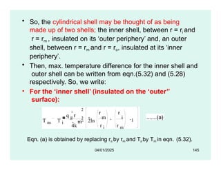
145.
• So, thecylindrical shell may be thought of as being
made up of two shells; the inner shell, between r = ri and
r = rm , insulated on its ‘outer periphery’ and, an outer
shell, between r = rm and r = ro, insulated at its ‘inner
periphery’.
• Then, max. temperature difference for the inner shell and
outer shell can be written from eqn.(5.32) and (5.28)
respectively. So, we write:
• For the ‘inner shell’ (insulated on the ‘outer’’
surface):
T m T i
q g
r
4k r i
2ln
r r
r m
m i 1
2
2
m
.......(a)
04/01/2025 145
Eqn. (a) is obtained by replacing ro by rm and Toby Tm in eqn. (5.32).
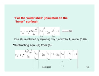
146.
•For the ‘outershell’ (insulated on the
‘inner’’ surface):
T m T o
q g
r
4k
2
o
r o
r m r m
2ln
r 1
2
m
............(b)
Eqn. (b) is obtained by replacing ri by rm and Ti by Tm in eqn. (5.28).
•Subtracting eqn. (a) from (b):
T i T o
q g
r 2
m
4k
r o
r m
2
2ln
r o
r m
1 2ln
r m
r i
r i
r m
2
1
04/01/2025 146
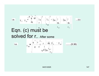
147.
i.e. T iT o
q r 2
g m
4k
r o
r
m
2
r i
r m
2
2ln
r
m
r o
2ln
r
m
r i
....(c)
Eqn. (c) must be
solved for rm. After some
manipulation, we get:
i.e.
r m
q r
2
2
g o i
r 4k T i T o
g
r i
q 2ln
r o
........(5.36)
04/01/2025 147
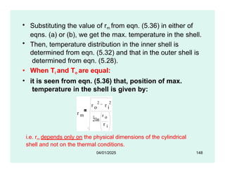
148.
• Substituting thevalue of rm from eqn. (5.36) in either of
eqns. (a) or (b), we get the max. temperature in the shell.
• Then, temperature distribution in the inner shell is
determined from eqn. (5.32) and that in the outer shell is
determined from eqn. (5.28).
• When Ti and To are equal:
• it is seen from eqn. (5.36) that, position of max.
temperature in the shell is given by:
r m
r r
o i
2 2
2ln
r o
r i
i.e. rm depends only on the physical dimensions of the cylindrical
shell and not on the thermal conditions.
04/01/2025 148
149.
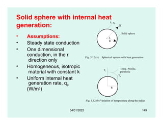
Solid sphere withinternal heat
generation: Q
Ti
To
k, qg
Fig. 5.12 (a) Spherical system with heat generation
L
R
Solid sphere
• Assumptions:
• Steady state conduction
• One dimensional
conduction, in the r
direction only
• Homogeneous, isotropic
material with constant k
• Uniform internal heat
generation rate, qg
(W/m3)
To
Fig. 5.12 (b) Variation of temperature along the radius
R
Temp. Profile,
parabolic
Tw
04/01/2025 149
150.
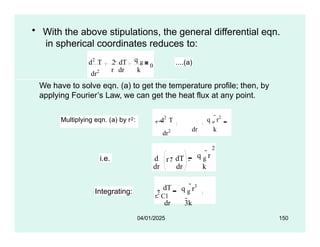
• With theabove stipulations, the general differential eqn.
in spherical coordinates reduces to:
dr2
d2
T 2 dT
r dr k
q g
0 ....(a)
We have to solve eqn. (a) to get the temperature profile; then, by
applying Fourier’s Law, we can get the heat flux at any point.
Multiplying eqn. (a) by r2: d2
T
dT
q g
r2
r
2 2r0
dr2 dr k
i.e. r
dr dr
d 2 dT
2
q g
r
k
Integrating:
dT q g
r3
dr 3k
r
2 C1
04/01/2025 150
151.
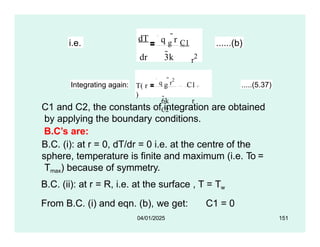
i.e.
dT
dr 3k
q g
rC1
r
2
......(b)
Integrating again: T( r
)
q g
r
2
C1
6k r
C2
.....(5.37)
C1 and C2, the constants of integration are obtained
by applying the boundary conditions.
B.C’s are:
B.C. (i): at r = 0, dT/dr = 0 i.e. at the centre of the
sphere, temperature is finite and maximum (i.e. To =
Tmax) because of symmetry.
B.C. (ii): at r = R, i.e. at the surface , T = Tw
From B.C. (i) and eqn. (b), we get: C1 = 0
04/01/2025 151
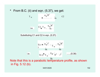
152.
• From B.C.(ii) and eqn. (5.37), we get:
q g
R2
T w
6k
C2
i.e.
q g
R2
C2 T w
6k
Substituting C1 and C2 in eqn. (5.37):
T( r
)
q g
r2
6k
T w
q g
R2
6k
i.e.
T( r) T w
q g
6k
R2
r2 .......(5.38)
04/01/2025 152
Note that this is a parabolic temperature profile, as shown
in Fig. 5.12 (b).
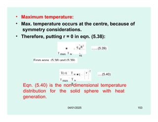
153.
• Maximum temperature:
•Max. temperature occurs at the centre, because of
symmetry considerations.
• Therefore, putting r = 0 in eqn. (5.38):
q g
R2
T max T w 6k
.......(5.39)
From eqns. (5.38) and (5.39),
T( r) T w
T max
1
r
T w
R
2
.....(5.40)
04/01/2025 153
Eqn. (5.40) is the non-dimensional temperature
distribution for the solid sphere with heat
generation.
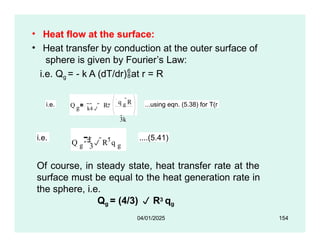
154.
• Heat flowat the surface:
• Heat transfer by conduction at the outer surface of
sphere is given by Fourier’s Law:
i.e. Qg = - k A (dT/dr)at r = R
i.e. Q g R
k4
q g
R
3k
2 ...using eqn. (5.38) for T(r
i.e.
3
Q g
4 R3 q g
....(5.41)
04/01/2025 154
Of course, in steady state, heat transfer rate at the
surface must be equal to the heat generation rate in
the sphere, i.e.
Qg = (4/3) R3 qg
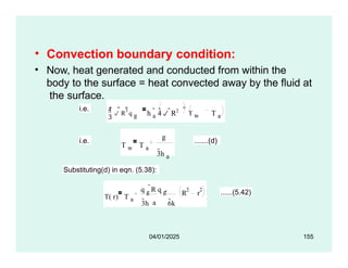
155.
• Convection boundarycondition:
• Now, heat generated and conducted from within the
body to the surface = heat convected away by the fluid at
the surface.
i.e.
4 R
3 q g h a
4 R2
T a
T w
i.e.
T w T a
g
3h a
.......(d)
Substituting(d) in eqn. (5.38):
T( r) T a
a
3h 6k
R r
2 2
q g
R q g ......(5.42)
04/01/2025 155
156.
Again, for max.temp. put r = 0 in eqn. (5.42):
T max T a a
q g
R q g
R2
3h 6k
.......(5.43)
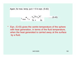
• Eqn. (5.43) gives the centre temperature of the sphere
with heat generation, in terms of the fluid temperature,
when the heat generated is carried away at the surface
by a fluid.
04/01/2025 156
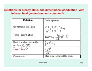
157.
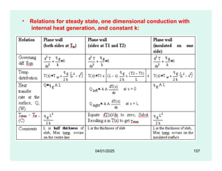
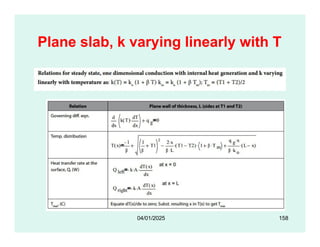
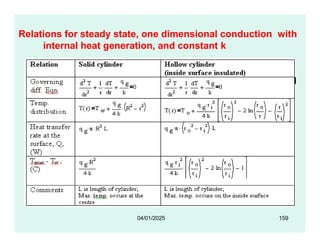
• Relations forsteady state, one dimensional conduction with
internal heat generation, and constant k:
04/01/2025 157
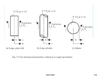
TRANSIENT HEAT CONDUCTION:
04/01/2025173
• In transient conduction, temperature depends
not only on position in the solid, but also on
time.
• So, mathematically, this can be written as T =
T(x,y,z,), where represents the time
coordinate.
• Typical examples of transient
conduction:
• heat exchangers
• boiler tubes
• cooling of I.C.Engine cylinder heads
174.
Examples (contd.):
04/01/2025 174
•heat treatment of engineering
components and quenching of ingots
• heating of electric irons
• heating and cooling of buildings
• freezing of foods, etc.
175.
Lumped system analysis
(Newtonianheating or cooling):
• In lumped system analysis, the internal
conduction resistance of the body to heat
flow (i.e. L/(k.A)) is negligible compared
to the convective resistance (i.e. 1/(h.A))
at the surface.
• So, the temperature of the body, no doubt,
varies with time, but at any given instant,
the temperature within the body is uniform
and is independent of position. i.e. T =
T() only.
04/01/2025 175
176.
Lumped system analysis
(Newtonianheating or cooling):
• Practical examples of such cases are:
heat treatment of small metal pieces,
measurement of temperature with a
thermocouple or thermometer etc, where
the internal resistance of the object for
heat conduction may be considered as
negligible.
04/01/2025 176
177.
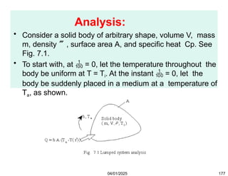
Analysis:
• Consider asolid body of arbitrary shape, volume V, mass
m, density , surface area A, and specific heat Cp. See
Fig. 7.1.
• To start with, at = 0, let the temperature throughout the
body be uniform at T = Ti. At the instant = 0, let the
body be suddenly placed in a medium at a temperature of
Ta, as shown.
04/01/2025 177
178.
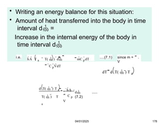
• Writing anenergy balance for this situation:
• Amount of heat transferred into the body in time
interval d =
Increase in the internal energy of the body in
time interval d
i.e.
hA T a T( ) d mC p
dT
C p
VdT
....(7.1) since m = .
V
dT d T( ) T a
Now, since Ta is a constant, we can write:
Therefore,
d T( ) T a
T( ) T
a
hA
C p
V
d .....
(7.2)
04/01/2025 178
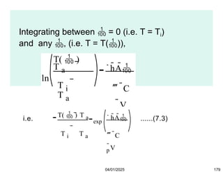
179.
Integrating between = 0 (i.e. T = Ti)
and any , (i.e. T = T()),
T( )
T a
ln
T i
T a
hA
C
p
V
i.e.
T( ) T a
T i T a
exp
hA
C
p
V
......(7.3)
04/01/2025 179
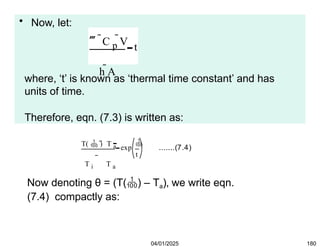
180.
• Now, let:
C p
V
h A
t
where, ‘t’ is known as ‘thermal time constant’ and has
units of time.
Therefore, eqn. (7.3) is written as:
T( ) T a
T i T a
exp
t
.......(7.4)
04/01/2025 180
Now denoting θ = (T() – Ta), we write eqn.
(7.4) compactly as:
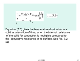
181.
i
T( )T a
T i T a
exp
t
......(7.5)
04/01/2025 181
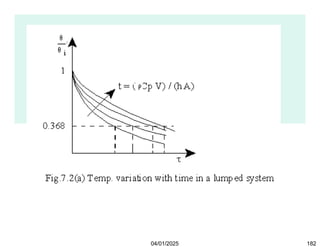
Equation (7.5) gives the temperature distribution in a
solid as a function of time, when the internal resistance
of the solid for conduction is negligible compared to
the convective resistance at its surface. See Fig. 7.2
(a)
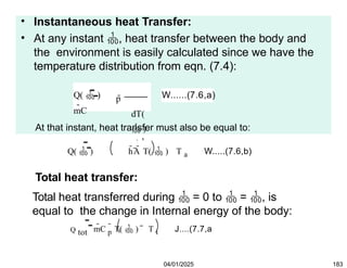
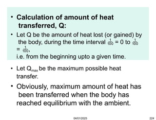
• Instantaneous heatTransfer:
• At any instant , heat transfer between the body and
the environment is easily calculated since we have the
temperature distribution from eqn. (7.4):
p
Q( )
mC
dT(
)
d
W......(7.6,a)
At that instant, heat transfer must also be equal to:
Q( ) hA T( ) T a W.....(7.6,b)
Total heat transfer:
Total heat transferred during = 0 to = , is
equal to the change in Internal energy of the body:
Q tot mC p
T( ) T i J....(7.7,a
04/01/2025 183
184.
Q tot
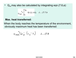
• Qtotmay also be calculated by integrating eqn.(7.6,a):
Q( ) d J.....(7.7,b
0
Max. heat transferred:
When the body reaches the temperature of the environment,
obviously maximum heat has been transferred:
Q max mC p T a T i J.....(7.8
04/01/2025 184
If Qmax is negative, it means that the body has lost heat,
and if Qmax is positive, then body has gained heat.
185.
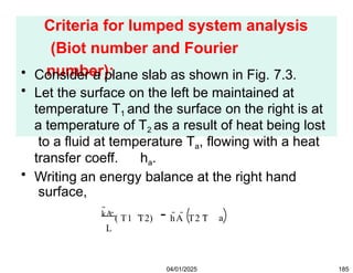
Criteria for lumpedsystem analysis
(Biot number and Fourier
number):
• Consider a plane slab as shown in Fig. 7.3.
• Let the surface on the left be maintained at
temperature T1 and the surface on the right is at
a temperature of T2 as a result of heat being lost
to a fluid at temperature Ta, flowing with a heat
transfer coeff. ha.
• Writing an energy balance at the right hand
surface,
a
kA ( T1 T2) hA T2 T
L
04/01/2025 185
186.
Criteria for lumpedsystem analysis
(Biot number and Fourier
number):
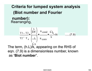
Rearranging,
T1 T2
T2 T a 1
h A
R conv
k
L
kA R cond h L
Bi ......(7.9)
04/01/2025 186
The term, (h.L)/k, appearing on the RHS of
eqn. (7.9) is a dimensionless number, known
as ‘Biot number’.
187.
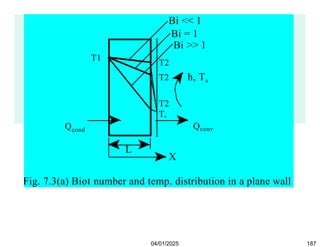
Fig. 7.3(a) Biotnumber and temp. distribution in a plane wall
X
T1
T2 h, Ta
T2
Ta
Bi << 1
Bi = 1
Bi >> 1
T2
Qconv
Qcond
L
04/01/2025 187
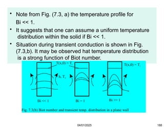
188.
• Note fromFig. (7.3, a) the temperature profile for
Bi << 1.
• It suggests that one can assume a uniform temperature
distribution within the solid if Bi << 1.
• Situation during transient conduction is shown in Fig.
(7.3,b). It may be observed hat temperature distribution
is a strong function of Biot number.
Fig. 7.3(b) Biot number and transient temp. distribution in a plane wall
h, Ta
Bi << 1 Bi = 1 Bi >> 1
T(x,0) = Ti T(x,0) = Ti
04/01/2025 188
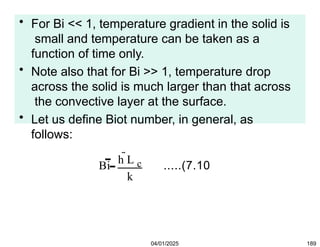
189.
• For Bi<< 1, temperature gradient in the solid is
small and temperature can be taken as a
function of time only.
• Note also that for Bi >> 1, temperature drop
across the solid is much larger than that across
the convective layer at the surface.
• Let us define Biot number, in general, as
follows:
Bi
h L c
k
.....(7.10
04/01/2025 189
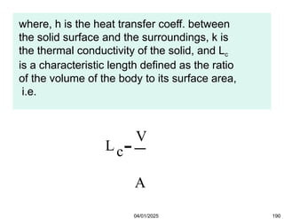
190.
where, h isthe heat transfer coeff. between
the solid surface and the surroundings, k is
the thermal conductivity of the solid, and Lc
is a characteristic length defined as the ratio
of the volume of the body to its surface area,
i.e.
Lc
V
A
04/01/2025 190
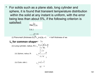
191.
• For solidssuch as a plane slab, long cylinder and
sphere, it is found that transient temperature distribution
within the solid at any instant is uniform, with the error
being less than about 5%, if the following criterion is
satisfied: hL c
Bi
0.1
......(7.11
k
Lc for common shapes:
(i) Plane wall (thickness 2L): L c A 2L
2A
L = half thickness of wa
(ii) Long cylinder, radius, R: L c
2 RL
R2 L R
2
(iii) Sphere, radius, R:
L c
4 R3
3
4 R2
R
3
(iv) Cube, side L: L c
L
3
6L2
L
6
04/01/2025 191
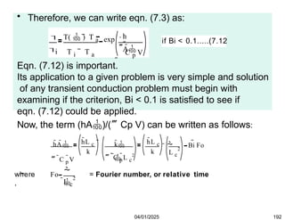
192.
• Therefore, wecan write eqn. (7.3) as:
i
T( ) T a
T i T a
h
A
C p V
exp
if Bi < 0.1.....(7.12
Eqn. (7.12) is important.
Its application to a given problem is very simple and solution
of any transient conduction problem must begin with
examining if the criterion, Bi < 0.1 is satisfied to see if
eqn. (7.12) could be applied.
Now, the term (hA)/(Cp V) can be written as follows:
hA
C p
V C p
L c
2
hL c hL c
k k 2
L c
k
Bi Fo
where
,
Fo
2
L c
= Fourier number, or relative time
04/01/2025 192
193.
• Fourier number,like Biot number, is an
important parameter in transient heat
transfer problems.
• It is also known as ‘dimensionless time’.
• Fourier number signifies the degree of
penetration of heating or cooling
effect through a solid.
• For small Fo, large will be required to
get significant temperature changes.
04/01/2025 193
194.
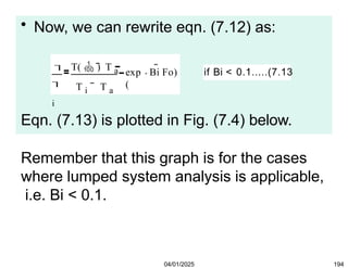
• Now, wecan rewrite eqn. (7.12) as:
i
T( ) T a
T i T a
exp
(
Bi Fo) if Bi < 0.1.....(7.13
04/01/2025 194
Eqn. (7.13) is plotted in Fig. (7.4) below.
Remember that this graph is for the cases
where lumped system analysis is applicable,
i.e. Bi < 0.1.
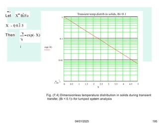
195.
Let X BiFo
X0 0.1 5
Then
i
exp( X)
exp( X)
X
0 0.5 1 1.5 2 2.5 3 3.5 4 4.5 5
1 10
3
0.01
0.1
1
Transient temp.distrib.in solids, Bi<0.1
04/01/2025 195
Fig. (7.4) Dimensionless temperature distribution in solids during transient
transfer, (Bi < 0.1)--for lumped system analysis
196.
Response time ofa thermocouple:
04/01/2025 196
• Lumped system analysis is usefully
applied in the case of temperature
measurement with a thermometer or a
thermocouple. Obviously, it is desirable
that the thermocouple indicates the source
temperature as fast as possible.
• ‘Response time’ of a thermocouple is
defined as the time taken by it to reach the
source temperature.
197.
Response time ofa thermocouple:
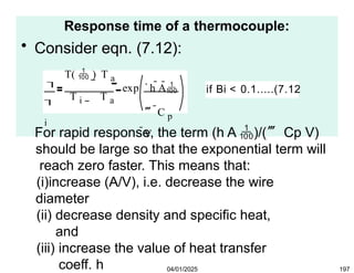
• Consider eqn. (7.12):
i
T( ) T a
exp
T i T a
h A
C p
V
if Bi < 0.1.....(7.12
04/01/2025 197
For rapid response, the term (h A )/( Cp V)
should be large so that the exponential term will
reach zero faster. This means that:
(i)increase (A/V), i.e. decrease the wire
diameter
(ii) decrease density and specific heat,
and
(iii) increase the value of heat transfer
coeff. h
198.
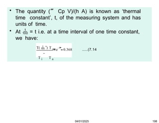
• The quantity( Cp V)/(h A) is known as ‘thermal
time constant’, t, of the measuring system and has
units of time.
• At = t i.e. at a time interval of one time constant,
we have:
T( ) T a
T i T a
1
e 0.368 .....(7.14
04/01/2025 198
From eqn. (7.14), it is clear that after an interval of time
equal to one time constant of the given temperature
measuring system, the temperature difference between the
body (thermocouple) and the source would be 36.8% of
the initial temperature difference. i.e. the temperature
difference would be reduced by 63.2%.
199.
Time required bya thermocouple to attain
63.2% of the value of initial temperature
difference is called its ‘sensitivity’.
For good response, obviously the response
time of thermocouple should be low.
As a thumb rule, it is recommended that while
using a thermocouple to measure temperatures,
reading of the thermocouple should be taken
after a time equal to about four time periods has
elapsed.
04/01/2025 199
200.
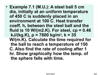
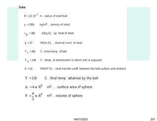
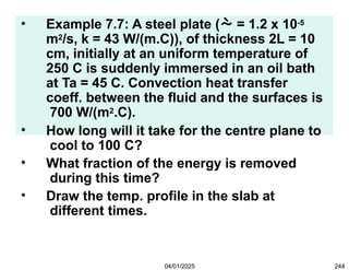
• Example 7.1(M.U.): A steel ball 5 cm
dia, initially at an uniform temperature
of 450 C is suddenly placed in an
environment at 100 C. Heat transfer
coeff. h, between the steel ball and the
fluid is 10 W/(m2.K). For steel, cp = 0.46
kJ/(kg.K), ρ = 7800 kg/m3, k = 35
W/(m.K). Calculate the time required for
the ball to reach a temperature of 150
C. Also find the rate of cooling after 1
hr. Show graphically how the temp. of
the sphere falls with time.
04/01/2025 200
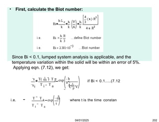
• First, calculatethe Biot number:
Since Bi < 0.1, lumped system analysis is applicable, and the
temperature variation within the solid will be within an error of 5%.
Applying eqn. (7.12), we get:
i
T( ) T a
T T
i a
h
A
C p V
exp
if Bi < 0.1.....(7.12
i.e.
T T a
T i T a
exp
t
where t is the time constan
04/01/2025 202
203.
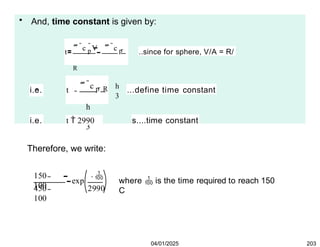
• And, timeconstant is given by:
t
c p
V c p
R
Ah h
3
..since for sphere, V/A = R/
i.e. t c p R
h
3
...define time constant
i.e. t 2990 s....time constant
Therefore, we write:
150
100
450
100
exp
2990
where is the time required to reach 150
C
04/01/2025 203
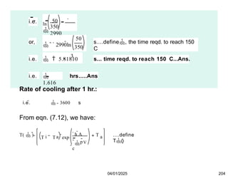
204.
i.e. ln
50
350
2990
or,
50
350
2990ln
s....define,the time reqd. to reach 150
C
i.e.
3
5.81810 s... time reqd. to reach 150 C...Ans.
i.e.
1.616
hrs.....Ans
Rate of cooling after 1 hr.:
i.e. 3600 s
From eqn. (7.12), we have:
T( ) i a
h A
p
c
V
T T exp
T a ....define
T()
04/01/2025 204
205.
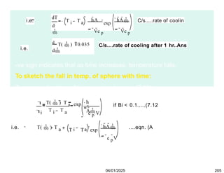
i.e.
dT
d
i
T T a
hA
Vc p
hA
Vc p
exp
C/s.....rate of coolin
d
T( ) 0.035
d
C/s....rate of cooling after 1 hr..Ans
i.e.
-ve sign indicates that as time increases, temperature falls.
To sketch the fall in temp. of sphere with time:
Temp. as a function of time is given by eqn. (7.12):
i
T( ) T a
T T
i a
h
A
c p V
exp
if Bi < 0.1.....(7.12
i.e. T( ) T a i a
hA
c p
V
T T exp ....eqn. (A
04/01/2025 205
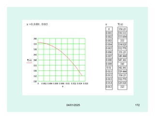
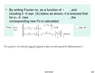
206.
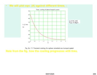
• We willplot eqn. (A) against different times, :
0 0.5 1 1.5 2
2.5 3 3.5 4
500
450
400
350
T( 3600)
300
250
200
150
100
Trans. cooling of sphere-lumped system
in hrs. and
T() in deg.C
Fig. Ex. 7.1 Transient cooling of a sphere considred as a lumped system
04/01/2025 206
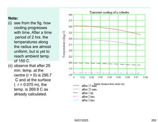
Note from the fig. how the cooling progresses with time.
After about 4 hrs. duration, the sphere approaches the temp.
of the ambient.
You can also verify from the graph that the time required for the
sphere to reach 150 C is 1.616 hrs, as calculated earlier.
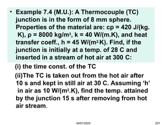
207.
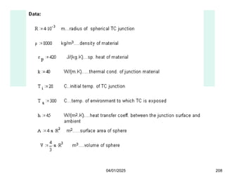
• Example 7.4(M.U.): A Thermocouple (TC)
junction is in the form of 8 mm sphere.
Properties of the material are: cp = 420 J/(kg.
K), ρ = 8000 kg/m3, k = 40 W/(m.K), and heat
transfer coeff., h = 45 W/(m2.K). Find, if the
junction is initially at a temp. of 28 C and
inserted in a stream of hot air at 300 C:
(i) the time const. of the TC
(ii)The TC is taken out from the hot air after
10 s and kept in still air at 30 C. Assuming ‘h’
in air as 10 W/(m2.K), find the temp. attained
by the junction 15 s after removing from hot
air stream.
04/01/2025 207
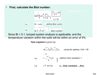
• First, calculatethe Biot number:
Bi h L c
4 R2
4 ( ) R3
h V h 3
k k A k
i.e. Bi h R
k 3
...define Biot numb
i.e.
Bi 1.5 10 3 ...Biot number
Since Bi < 0.1, lumped system analysis is applicable, and the
temperature variation within the solid will be within an error of 5%.
See Fig. Ex. 7.4 (a).
Time constant is given by:
t
c p
V c p
R
A h h
3
..since for sphere, V/A = R/
i.e.
c p R
t ...define time constant, t
h 3
i.e. t 99.556 s....time constant.....Ans.
04/01/2025 209
210.
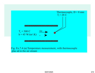
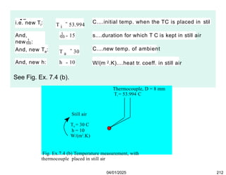
Fig. Ex.7.4 (a)Temperature measurement, with thermocouple
plac ed in the air stream
Thermocouple, D = 8 mm
Ti = 28 C
Ta = 300 C Air
h = 45 W/(m2
.K)
04/01/2025 210
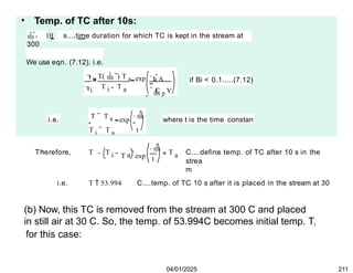
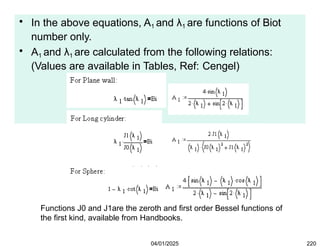
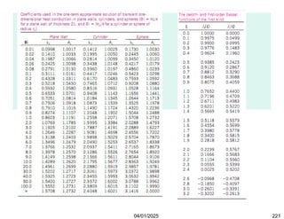
211.
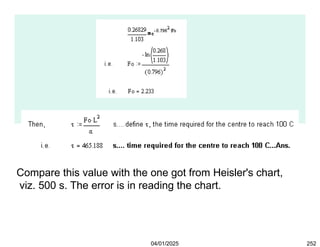
• Temp. ofTC after 10s:
10 s....time duration for which TC is kept in the stream at
300
We use eqn. (7.12). i.e.
i
T( ) T a
T T
i a
h A
C p V
exp
if Bi < 0.1.....(7.12)
i.e.
T T a
exp
T i T a t
where t is the time constan
Therefore, T T i a
t
T exp a
T C....define temp. of TC after 10 s in the
04/01/2025 211
strea
m
i.e. T 53.994 C....temp. of TC 10 s after it is placed in the stream at 30
(b) Now, this TC is removed from the stream at 300 C and placed
in still air at 30 C. So, the temp. of 53.994C becomes initial temp. Ti
for this case:
212.
i.e. new Ti:T i 53.994
C....initial temp. when the TC is placed in stil
And,
new:
15 s....duration for which T C is kept in still air
And, new Ta: T a 30
C....new temp. of ambient
And, new h: h 10 W/(m 2.K)....heat tr. coeff. in still air
See Fig. Ex. 7.4 (b).
Thermocouple, D = 8 mm
Ti = 53.994 C
Still air
Ta = 30 C
h = 10
W/(m2
.K)
Fig. Ex.7.4 (b) Temperature measurement, with
thermocouple placed in still air
04/01/2025 212
213.
And, new timeconstant:
i.e. t
c p R
h
3
...define time constant
i.e. t 448 s....tim e constant
Therefore, i a
t
T T T exp a
T C....define temp. of T C after 15 s in still
04/01/2025 213
i.e. T 53.204 C....temp. of TC 15 s after it is placed in still air
at 30 C...Ans.
214.
One-dimensional transient conductionin large
plane walls, long cylinders and spheres when
Biot number > 0.1:
• When the temperature gradient in the solid is not
negligible (i.e. Bi > 0.1), lumped system analysis
is not applicable.
• One term approximation solutions:
• Fig. 7.6 shows schematic diagram and
coordinate systems for a large, plane slab, long
cylinder and a sphere.
• Consider a plane slab of thickness 2L, shown in
Fig (a) above. Initially, i.e. at = 0, the slab is
at an uniform temperature, Ti.
04/01/2025 214
215.
One-dimensional transient conductionin large
plane walls, long cylinders and spheres when
Biot number > 0.1:
• Suddenly, at = 0, both the surfaces of the slab
are subjected to convection heat transfer with
an ambient at temperature Ta , with a heat
transfer coeff. h, as shown.
• Because of symmetry, we need to consider only
half the slab, and that is the reason why we
chose the origin of the coordinate system on the
mid-plane.
• Then, we can write the mathematical formulation
of the problem for plane slab as follows:
04/01/2025 215
2
dx2
d T 1 dT
d
in 0< x <L, for > 0.......(7.23,
a
dT
dx
0 at x = 0, for > 0.......(7.23,
b)
k dT
dx
h T T a at x = L, for > 0 ......(7.23,
c)
T T i
for = 0, in 0 < x < L .....(7.23,
d)
04/01/2025 217
The solution of the above problem, however, is rather
involved and consists of infinite series. So, it is more
convenient to present the solution either in tabular form or
charts.
For this purpose, we define the following dimensionless parameters:
218.
• While usingthe tabular or chart solutions, note one
important difference in defining Biot number:
• Characteristic length in Biot number is taken as half
thickness L for a plane wall, Radius R for a long
cylinder and sphere instead of being calculated as
V/A, as done in lumped system analysis.
(i) Dimensionless temperature:
T( x )
T a
( x )
T i
T a
(ii) Dimensionless distance from the centre: X
x
L
(iii) Dimensionless heat transfer coefficient: Bi hL
k
...Biot number
(iv) Dimensionless time:
Fo
L
2
....Fourier number
04/01/2025 218
219.
• It isobserved that for Fo > 0.2, considering only the first
term of the series and neglecting other terms, involves
an error of less than 2%.
• Generally, we are interested in times, Fo > 0.2.
• So, it becomes very useful and convenient to use one
term approximation solution, for all these three cases,
as follows:
Plane wall:
T( x ) T a
T i T a
( x ) A 1 e
1
2
Fo
1
x
cos
L
...Fo > 0.2....(7.24, a
Long cylinder: T( r ) T a
T i T a
( x ) A 1 e
1
2
Fo
J 0
1 r
R
...Fo > 0.2....(7.24, b
sphere:
T( r ) T a
T i T a
1
( x ) A 1
e
1
r
2 Fo
sin
R
1
r
R
...Fo > 0.2....(7.24, c
04/01/2025 219
220.
• In theabove equations, A1 and λ1 are functions of Biot
number only.
• A1 and λ1 are calculated from the following relations:
(Values are available in Tables, Ref: Cengel)
Functions J0 and J1are the zeroth and first order Bessel functions of
the first kind, available from Handbooks.
04/01/2025 220
• Now, atthe centre of a plane wall, cylinder and sphere,
we have the condition x = 0 or r = 0.
• Then, noting that cos(0) = 1, J0 (0) = 1, and limit of
sin(x)/x is also 1, eqns. (7.24) become:
• At the centre of plane wall, cylinder and
sphere:
(x = 0)
Centre of plane wall:
0
T 0 T a
T T
i a
A 1 e
2
1
Fo
....(7.25, a
Centre of long cylinder:
(r = 0)
0
T 0 T a
T T
i a
A 1 e
2
1
Fo
...(7.25, b
Centre of sphere
(r = 0)
T 0
T a
: 0
T i
T a
A 1 e
2
1
Fo
...(7.25, c
04/01/2025 222
223.
Therefore, first stepin the solution is to
calculate the Biot number;
• Once the Biot number is known, constants A1
and λ1 are found out from Tables and then use
relations given in eqns. (7.24) and (7.25) to
calculate the temperature at any desired
location.
• The one-term solutions are presented in chart
form in the next section.
• But, generally, it is difficult to read these charts
accurately.
• So, relations given in eqns. (7.24) and (7.25)
along with Tables for A1 and λ1 should be
preferred to the charts.
04/01/2025 223
224.
• Calculation ofamount of heat
transferred, Q:
• Let Q be the amount of heat lost (or gained) by
the body, during the time interval = 0 to
= ,
i.e. from the beginning upto a given time.
• Let Qmax be the maximum possible heat
transfer.
• Obviously, maximum amount of heat has
been transferred when the body has
reached equilibrium with the ambient.
04/01/2025 224
225.
• i.e.
Q max VC p
T i T a mC p
T i T a J.....(7.26
where is the density, V is the volume, (V) is the
mass,
Cp is the specific heat of the body.
Based on the one term approximation discussed above,
(Q/ Qmax) is calculated for the three cases, from the
following:
Plane wall:
Q
Q max
1
0
1
sin 1 ......(7.27, a
Cylinder:
Q
1 2
Q max
J 1
1
0
1
.....(7.27, b
Sphere:
Q
1 3
0
Q max
sin 1 1
cos 1
3
1
.....(7.27, c
04/01/2025 225
226.
• Note:
• (i)Remember well the definition of Biot
number- i.e. Bi = (hL/k), where L is half
thickness of the slab, and Bi = (hR/k),
where R is the outer radius of the cylinder or
the
sphere.
• (ii) Foregoing results are equally applicable to
a plane wall of thickness L, insulated on one
side and suddenly subjected to convection at
the other side. This is so because, the
boundary condition dT/dx = 0 at x = 0 for the
mid-plane of a slab of thickness 2L (see eqn.
7.23, b), is equally applicable to a slab of
thickness L, insulated at x = 0.
04/01/2025 226
227.
• Note (contd.):
•(iii) These results are also applicable to
determine the temperature response of a
body when temperature of its surface is
suddenly changed to Ts . This case is
equivalent to having convection at the
surface with a heat transfer coeff., h = ∞;
now, Ta is replaced by the prescribed
surface temperature, Ts.
• Remember that these results are valid
for the situation where Fourier number,
Fo > 0.2.
04/01/2025 227
228.
Heisler and Grobercharts:
04/01/2025 228
• The one term approximation solutions
(eqn. (7.25)) were represented in graphical
form by Heisler in 1947. They were
supplemented by Grober in 1961, with
graphs for heat transfer (eqn. (7.27)).
• These graphs are shown in following
slides for plane wall, long cylinder and a
sphere, respectively.
229.
Heisler and Grobercharts:
04/01/2025 229
• About the charts:
• First chart in each of these figures gives the non-
dimensionalised centre temperature T0. i.e. at x
= 0 for the slab of thickness 2L, and at r = 0 for
the cylinder and sphere, at a given time .
• Temperature at any other position at the same
time , is calculated using the next graph,
called ‘position correction chart’.
• Third chart gives Q/Qmax.
How to usethese charts?
04/01/2025 239
• Procedure of using these charts to solve
a numerical problem is as follows:
• First of all, calculate Bi from the data, with the
usual definition of Bi i.e. Bi = (h.Lc)/k, where Lc
is the characteristic dimension, given as: Lc =
(V/A).
• i.e. Lc = L, half-thickness for a plane wall, Lc =
R/2 for a cylinder, and Lc=R/3 for a sphere.
• If Bi < 0.1, use lumped system analysis;
otherwise, go for one term approx. or chart
solution.
240.
How to usethese charts?
04/01/2025 240
• If Bi > 0.1, calculate the Biot number
again with the appropriate definition of Bi
i.e. Bi =(hL/k) for a plane wall where L is
half-thickness, and Bi = (hR/k) for a
cylinder or sphere, where R is the outer
radius. Also, calculate Fourier number,
Fo = ./L2 for the plane wall, and
Fo =
./R2 for a cylinder or sphere.
• To calculate the centre temperature, use
the first chart in the set given,
depending upon the geometry being
241.
• Fo ison the x-axis; draw a vertical line to intersect the
(1/Bi) line; from the point of intersection, move
horizontally to the left to the y-axis to read the value of
o = (To –Ta)/(Ti – Ta). Here, To is the centre
temperature, which can now be calculated since Ti
and Ta are known.
• To calculate the temperature at any other position, use
second fig. of the set, as appropriate:
• Enter the chart with 1/Bi on the x-axis, move vertically
up to intersect the (x/L) (or (r/R)) curve, and from the
point of intersection, move to the left to read on the y-
axis, the value of = (T –Ta)/(To – Ta). Here, T
is the desired temperature at the indicated position.
04/01/2025 241
242.
• To findout the amount of heat transferred Q,
during a particular time interval from the
beginning (i.e. = 0), use the third fig. of
the set, depending upon the geometry.
• Enter the x-axis with the value of (Bi2 .Fo) and
move vertically up to intersect the curve
representing the appropriate Bi, and move to
the left to read on the y-axis, the value of
Q/Qmax.
• Q is then easily found out since Qmax =
m.Cp.(Ti – Ta).
• And,Q = (Q/Qmax ). Qmax .
04/01/2025 242
243.
• Note thefollowing in connection with these
charts:
• These charts are valid for Fourier number Fo >
0.2
• Note from the ‘position correction charts’ that at
Bi < 0.1 (i.e. 1/Bi > 10), temperature within the
body can be taken as uniform, without
introducing an error of more than 5%. This was
precisely the condition for application of ‘lumped
system analysis’.
• It is difficult to read these charts accurately,
since logarithmic scales are involved; also, the
graphs are rather crowded with lines. So, use of
one term approximation with tabulated values
of A1 and 1 should be preferred.
04/01/2025 243
244.
• Example 7.7:A steel plate ( = 1.2 x 10⁻⁵
m2/s, k = 43 W/(m.C)), of thickness 2L = 10
cm, initially at an uniform temperature of
250 C is suddenly immersed in an oil bath
at Ta = 45 C. Convection heat transfer
coeff. between the fluid and the surfaces is
700 W/(m2.C).
• How long will it take for the centre plane to
cool to 100 C?
• What fraction of the energy is removed
during this time?
• Draw the temp. profile in the slab at
different times.
04/01/2025 244
• It isnoted that Biot number is > 0.1; so, lumped system analysis is
not applicable.
• We will adopt Heisler chart solution and then check the results from
one term approximation solution.
• To find the time reqd. for the centre to reach 100 C:
• For using the charts, Bi = hL/k, which is already calculated.
Fourier number: Fo
L
2
04/01/2025 246
247.
• Now, withthis value of , enter the y-axis of Fig. (7.7,a).
Move horizontally to intersect the 1/Bi = 1.229 line; from the
point of intersection, move vertically down to x-axis to read Fo
= 2.4.
04/01/2025 247
248.
• Surface temperature:
•At the surface, x/L =1. Enter
Fig. (7.7, b) on the x-axis
with a value of 1/Bi = 1.229,
move up to intersect the
curve of x/L = 1, then move
to left to read on y-axis the
value of Θ = 0.7
04/01/2025 248
249.
• Fraction ofmax. heat transferred, Q/Qmax:
• We will use Grober's chart, Fig. (7.7, c):
• We need Bi2Fo to enter the x-axis:
We get:
Bi2 Fo 1.59
With the value of 1.59, enter the x-axis of Fig. (7.7, c), move vertically
up to intersect the curve of Bi = 0.814, then move horizontally to
read Q/Qmax = 0.8
04/01/2025 249
250.
i.e. from Fig.(7.7, c), we get:
Q
Q max
0.8
i.e. 80% of the energy is remov ed by the time the centre temp. has reache
100 C.....Ans.
04/01/2025 250
251.
• Verify byone term approximation solution:
and
Therefore, eqn. (7.25, a) becomes:
04/01/2025 251
252.
Compare this valuewith the one got from Heisler's chart,
viz. 500 s. The error is in reading the chart.
04/01/2025 252
253.
Compare this withthe value of 83.5 C obtained earlier.
04/01/2025 253
254.
Fraction of max.heat transferred, Q/Qmax:
i.e. 75.9% of the energy is removed by the time the
centre temp. has reached 100 C.....Ans.
Compare this with the value of 80% obtained earlier;
again, the error is in reading the charts.
04/01/2025 254
255.
• To drawtemp. profile in the plate at different
times:
• We have, for temp. distribution at any location:
Plane wall:
T( x )
T a
( x )
T i
T a
A 1 e
1
1
x
cos
L
2Fo
...Fo > 0.2....(7.24, a
(x = 0)
And, Centre of plane wall:
0
T 0 T a
T T
i a
A 1 e
2
1
Fo
....(7.25, a
Fourie r number as a function
o:f
Fo(
)
L
2
...for slab
04/01/2025 255
256.
• By writingFourier no. as a function of , and
incuding it in eqn. (A) below as shown, it is ensured that
for each new , the
corresponding new Fo is calculated.
Then, T( x
)
T a T i T a
A 1
e
1
2 Fo ( )
if x 0
T a i
T T a 1
2 1
x
L
e
1 Fo ( )
cos
A
otherwis
e
.....eqn. (A
04/01/2025 256
257.
• Note thatthis
graph shows
temp.
distribution for
one half of
the plate; for
the other half,
the temp.
distribution will
be identical.
• (ii) See from the
fig. how cooling
progresses with
time. After a
time period of 25
min. the
temperatures in
the plate are
almost uniform
at 45 C.
04/01/2025 257
258.
• Example 7.8:A long, 15 cm diameter cylindrical shaft
made of stainless steel 304 (k = 14.9 W/(m.C), r = 7900
kg/m3, Cp = 477 J/(kg.C), and a = 3.95 x 10⁻⁶ m2/s),
comes out of an oven at an uniform temperature of 450
C. The shaft is then allowed to cool slowly in a
chamber at 150 C with an average heat transfer coeff.
of 85 W/(m2.C).
• (i) Determine the temperature at the centre of the shaft
25 min. after the start of the cooling process.
• (ii) Determine the surface temp.at that time, and
• (iii) Determine the heat transfer per unit length of the
shaft during this time period.
• (iv) draw the temp. profile along the radius for different
times
04/01/2025 258
Working with HeislerCharts is left a an exercise to students.
However, we shall solve the problem with one-term
approximation formulas for a cylinder:
04/01/2025 260
Note:
(i) see fromthe fig. how
cooling progresses
with time. After a time
period of 2 hrs. the
temperatures along
the radius are almost
uniform, but is yet to
reach ambient temp.
of 150 C.
(ii) observe that after 25
min. temp. at the
centre (r = 0) is 296.7
C and at the surface
( r = 0.075 m), the
temp. is 269.9 C as
already calculated.
04/01/2025 265
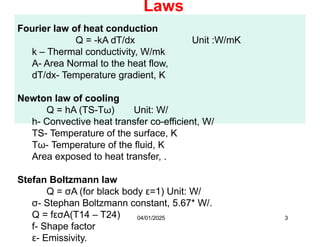
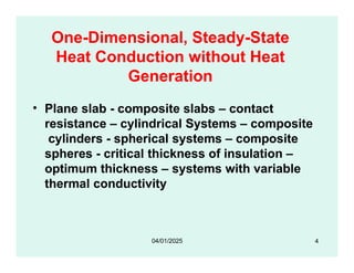
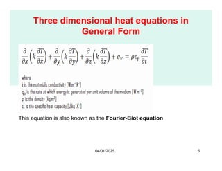
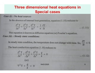
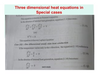
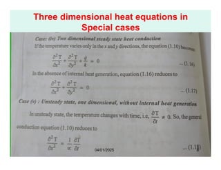
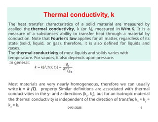
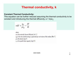
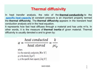
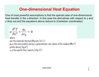
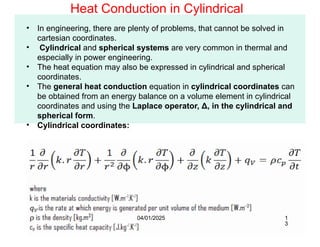
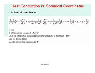
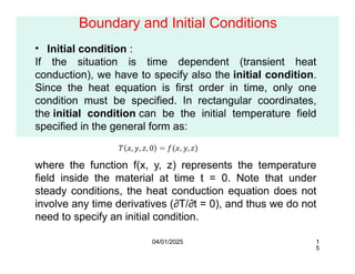
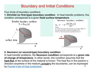
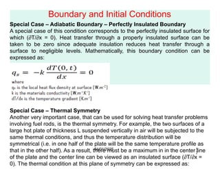
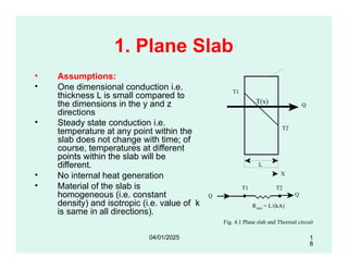
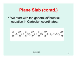
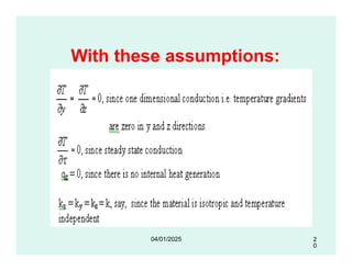
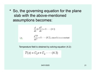
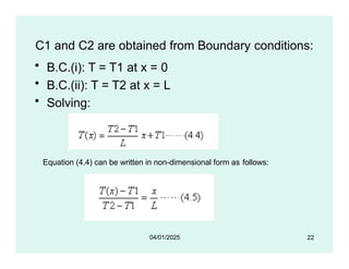
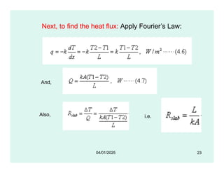
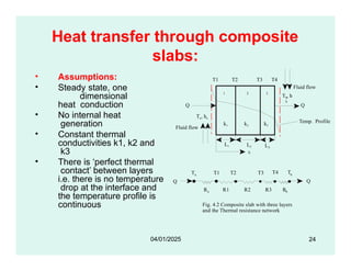
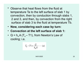
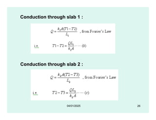
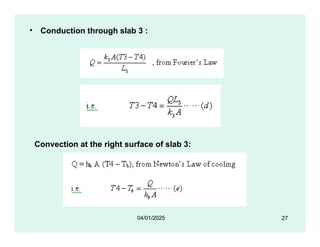
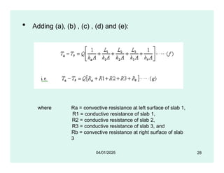
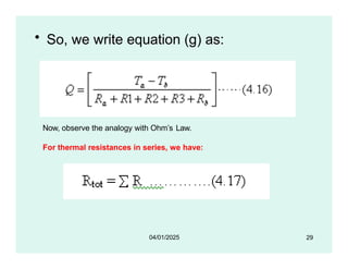
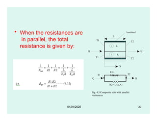
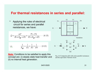
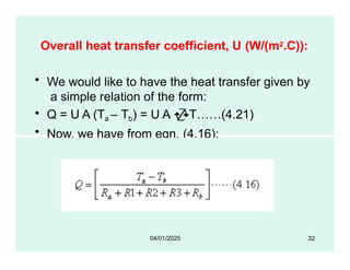
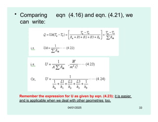
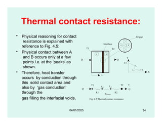
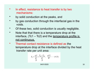
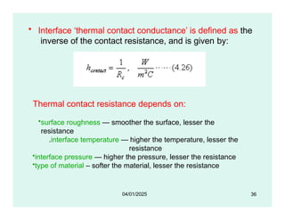
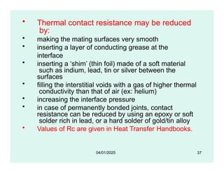
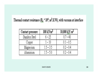
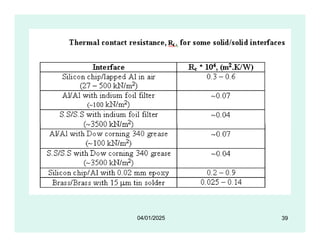
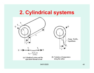
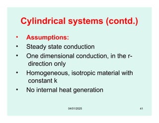
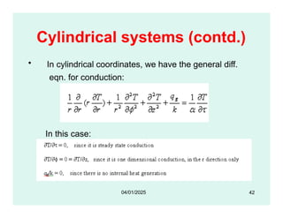
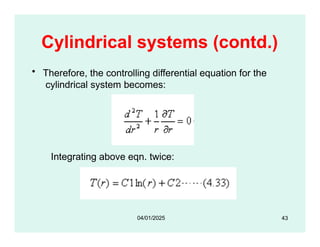
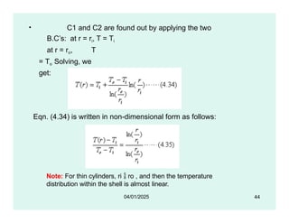
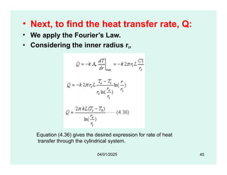
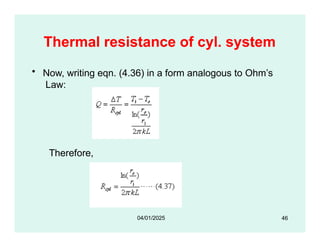
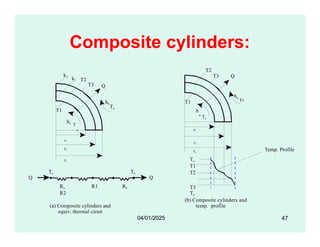
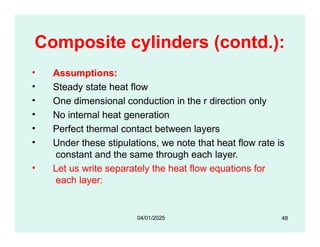
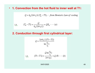
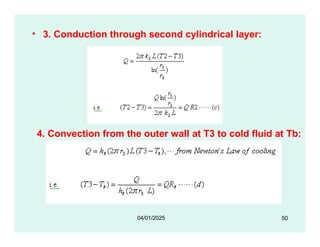
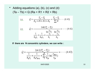
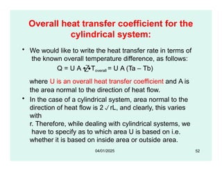
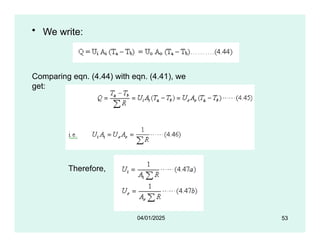
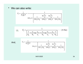
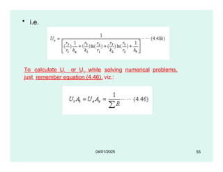
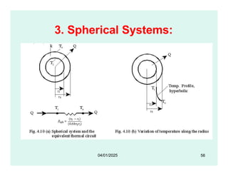
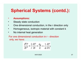
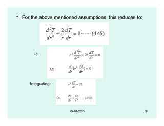
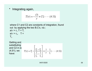
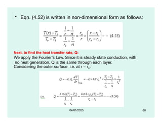
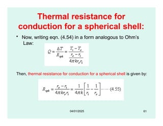
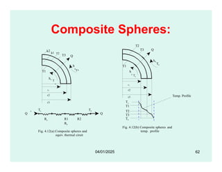
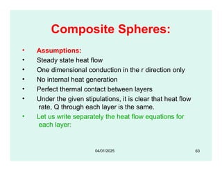
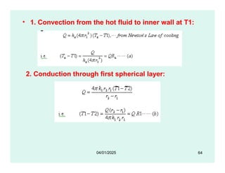
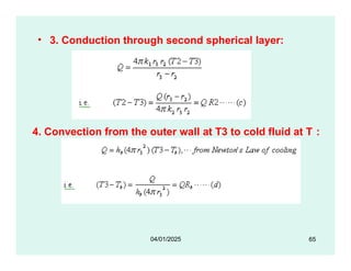
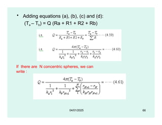
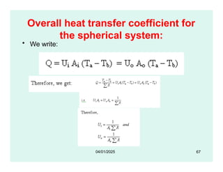
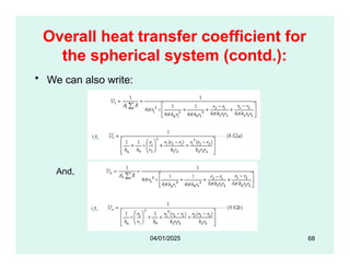
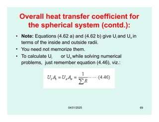
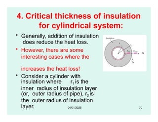
![Critical thickness of
insulation(contd.):
• Resistance to heat transfer is made up of two
components viz. conductive resistance through
the cylindrical insulation layer [ R= ln(r2/r1)/ (2 k
L) ] and convective resistance between the wall
surface and the surroundings [Ro = 1/(h. Ao )].
• As the insulation thickness is increased i.e. as
insulation radius r2 is increased, conductive
resistance of insulation increases; however,
convective resistance, given by [Ro =1/(h. Ao)]
goes on decreasing since Ao, the outside
surface area goes on increasing with
increasing radius.
71
04/01/2025](https://image.slidesharecdn.com/unit1conduction20-2-23-250401115504-b3088d0c/85/Unit-1-Conduction-one-dimensional-heat-condution-71-320.jpg)