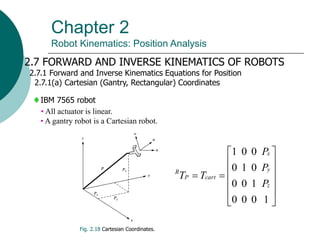
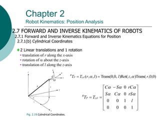
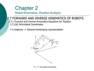
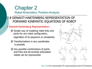
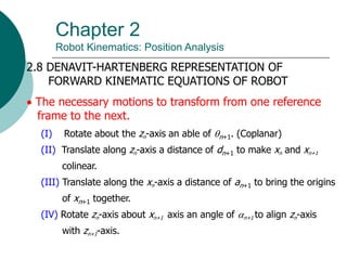
This document summarizes chapter 2 of a robotics textbook. It discusses robot kinematics including forward and inverse kinematics. Forward kinematics determines the robot's position given joint angles, while inverse kinematics calculates joint angles for a desired position. Several coordinate systems for representing robot positions are described, including Cartesian, cylindrical, and spherical coordinates. The Denavit-Hartenberg representation provides a standardized way to define the transformation between reference frames of successive robot links and joints, allowing calculation of forward kinematics for any robot configuration.
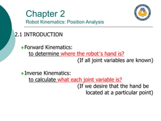
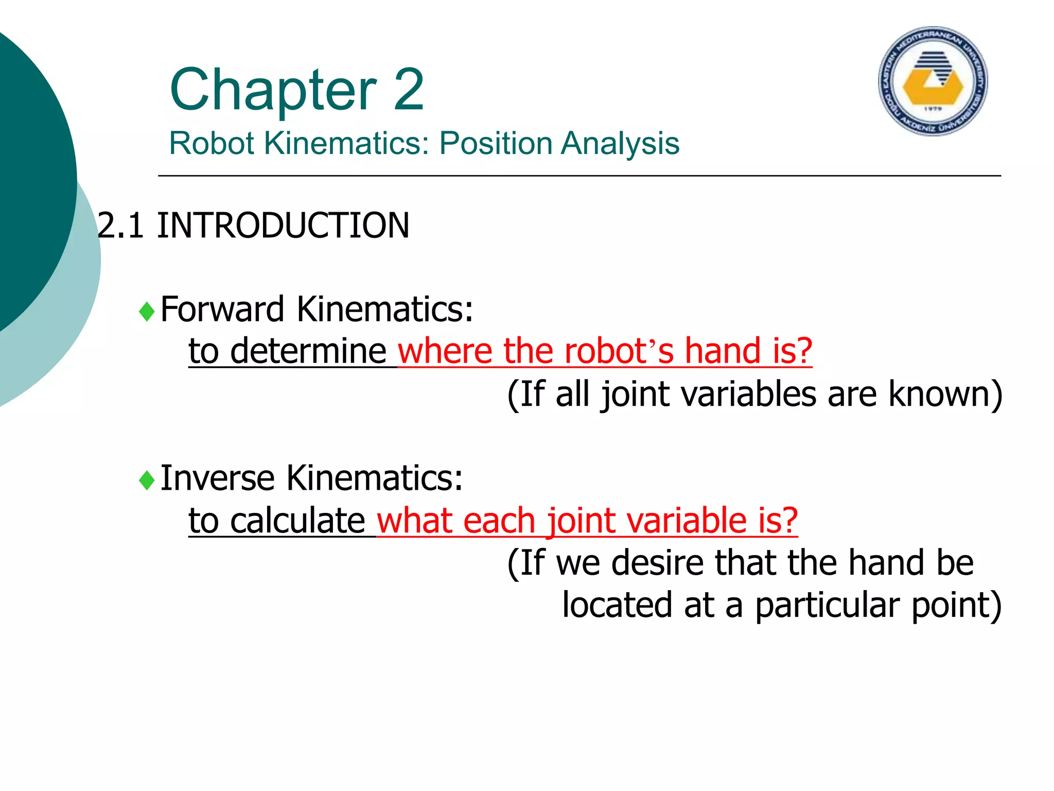


![Chapter 2
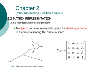
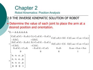
Robot Kinematics: Position Analysis
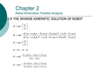
2.9 THE INVERSE KINEMATIC SOLUTION OF ROBOT
6
5
4
3
2
1
1
1
1 ]
[
1
0
0
0
A
A
A
A
A
RHS
A
p
a
o
n
p
a
o
n
p
a
o
n
A
z
z
z
z
y
y
y
y
x
x
x
x
6
5
4
3
2
1
1
1
1
1
0
0
0
1
0
0
0
0
0
0
1
0
0
0
0
A
A
A
A
A
p
a
o
n
p
a
o
n
p
a
o
n
C
S
S
C
z
z
z
z
y
y
y
y
x
x
x
x
](https://image.slidesharecdn.com/chapter2-robotkinematics-221012083348-dd71e75c/85/Chapter-2-Robot-Kinematics-ppt-31-320.jpg)