This document discusses increasing and decreasing functions, and optimization of functions of single and multiple variables. It defines increasing and decreasing functions using both simple definitions comparing function values as the independent variable changes, and using the sign of the derivative. Optimization of functions involves finding critical points where the first derivative is zero, and using the second derivative to determine if it is a maximum or minimum. Constrained optimization uses Lagrange multipliers to incorporate constraints. The Hessian determinant and bordered Hessian are discussed for determining maxima and minima of multivariable functions.

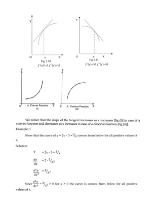
1. Curvature & Optimization
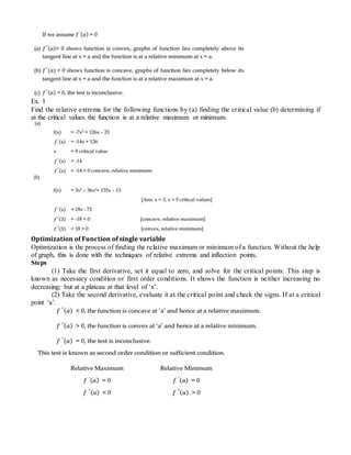
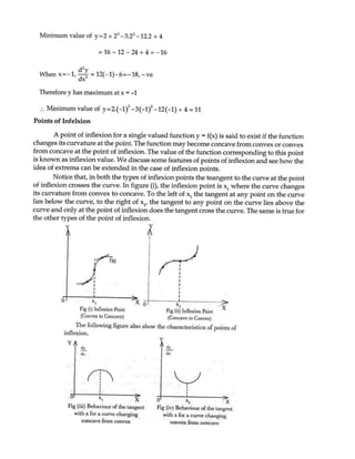
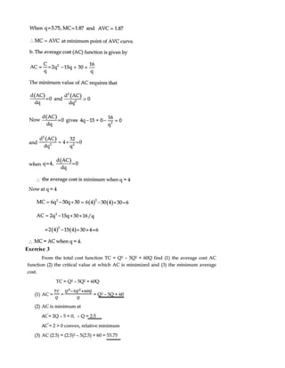
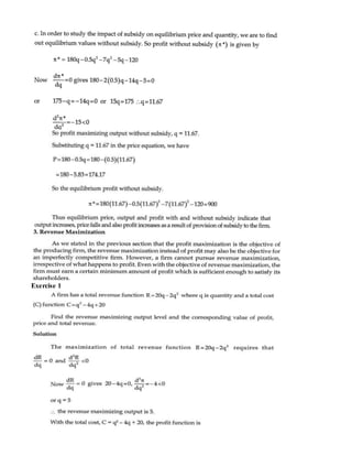
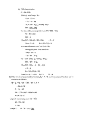
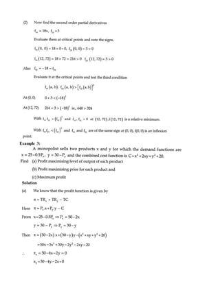
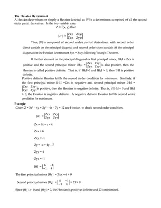
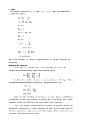
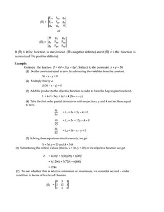
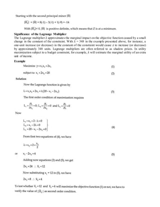
Increasing and Decreasing Functions
(a) Simple Definition: A function is an increasing function if the value of the function increases with
an increase in the value of the independent variable and decrease with a decrease in the value of the
independent variable.
For a function y = f(x)
When x1< x2 then f(x1) ≤ f(x2) the function is increasing
When x1< x2 then f(x1) < f(x2) the function is strictly increasing
A function is a decreasing function if the value of the function increases with a fall in the value of
independent variable and decrease with an increase in the value of independent variable.
For a function y = f(x)
When x1< x2 then f(x1) ≥ f(x2) the function is decreasing
When x1< x2 then f(x1) > f(x2) the function is strictly decreasing
(b) Definition Using Derivative: The derivative of a function can be applied to check whether given
function is an increasing function or decreasing function in a given interval.
If the sign of the first derivative is positive, it means that the value of the function f(x) increase
as the value of independent variable increases and vice versa. i.e. a function y = f(x) differentiable in
the interval [a, b] is said to be an increasing function if and only if its derivatives in an interval [a,
b] is non-negative. i.e.
A function y = f(x) differentiable in the interval [a, b] is said to be a decreasing function if and
only if its derivative in an interval [a, b] is non positive. i.e.
(c) Using Slope of tangent of a curve at a point: The derivative of a curve at a point also measures
the slope of the tangent to the curve at that point. If the derivative is positive, then it means that the
tangent has a positive slope and the function (curve) increases as the value of the independent
variable increase. Similar interpretation is given to the decreasing function and negative slope of
the tangent.
A function that increases or decreases over its entire domain is called monotonic function.

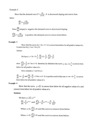
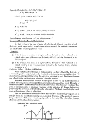
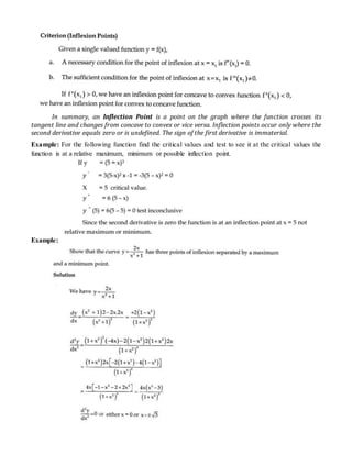
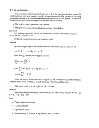
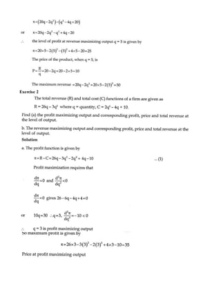
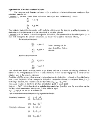
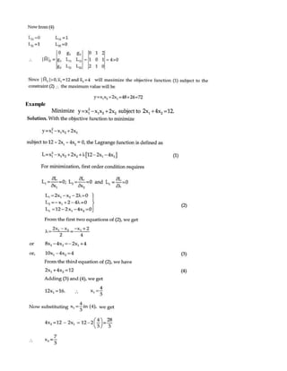
2. Example: Check whether the function 3x3 + 3x2 + x – 10 is increasing or decreasing?
The function is always positive because (3x+1)2 is positive since square of a real number is always
positive. Therefore the function is increasing.
Similarly, we have
(a) 2x2 – 5x + 10 is an Increasing function.
(b) x3– 10x2 + 2x + 5 is a Decreasing function.
A function is convex at x = a if in an area very close to [a, f(a)] the graph of the function lies completely
above its tangent line. Similarly a function f(x) is concave at x = a if in some small region close to the
point [a, f (a)] the graph of the function lies completely below its tangent line.

4. Example 3
Example 4

5. Example 5
Example 6
Relative Extrema
A relative extremum is a point at which a function is at a relative maximum or minimum. To be at a
relative maximum or minimum at a point ‘a’, the function must be at a relative ‘plateau’, i.e. neither
increasing nor decreasing at ‘a’. If the function is neither increasing nor decreasing at ‘a’, the first
derivative of the function at a must equal to zero or be undefined. A point in the domain of a function
where the derivative equals zero is called critical point of critical value. The second derivative is used to
distinguish between relative maximum and minimum mathematically.

6. Ex. 1
Find the relative extrema for the following functions by (a) finding the critical value (b) determining if
at the critical values the function is at a relative maximum or minimum.
Optimization of Function of single variable
Optimization is the process of finding the relative maximum or minimum of a function. Without the help
of graph, this is done with the techniques of relative extrema and inflection points.
Steps
(1) Take the first derivative, set it equal to zero, and solve for the critical points. This step is
known as necessary condition or first order conditions. It shows the function is neither increasing no
decreasing; but at a plateau at that level of ‘x’.
(2) Take the second derivative, evaluate it at the critical point and check the signs. If at a critical
point ‘a’.

8. Necessary Conditionfor Maximization/Minimizationofa function

9. Exercise
Exercise

11. In summary, an Inflection Point is a point on the graph where the function crosses its
tangent line and changes from concave to convex or vice versa. Inflection points occur only where the
second derivative equals zero or is undefined. The sign of the first derivative is immaterial.
Example: For the following function find the critical values and test to see it at the critical values the
function is at a relative maximum, minimum or possible inflection point.
Example:

12. Example:

14. Exercise 3

15. Exercise 1
Exercise 2

17. Exercise 3

18. Exercise 1

19. Exercise 2

20. Exercise 3
Find the maximum profits ‘π’ for a firm, given total revenue R = 4000Q – 33Q2 and the total cost
function C = 2Q3– 3Q2+ 400Q + 5000, assuming Q > 0.
Profit function: π= R – C
Π = (4000Q – 33Q2)– (2Q3– 3Q2+ 400Q + 5000)
= -2Q3– 30Q2+ 3600Q – 5000
Taking the first derivative, set it equal to zero, and solving this for Q we get critical points.
Taking the second derivative we get

21. Exercise 4
Given the total revenue R = 15Q – Q2 find the Average Revenue (AR), Marginal Revenue (MR) and the
level of output Q that maximizes Total Revenue (TR).
The output that maximize TR=7.5
AR when Q=7.5 is 15-7.5=7.5
MR when Q=7.5 is 15-2(7.5) =15-15=0
Exercise 5
From the total cost function TC = Q3– 5Q2 + 60Q find (1) the average cost AC function (2) the critical
value at which AC is minimized and (3) the minimum average cost.
Exercise 6
A producer has the possibility of discriminating between the domestic and foreign markets for a product
where the demands functions are Q1= 24 – 0.2P1 and Q2= 10 – 0.05P2; Where TC = 35 + 40Q, what
price will be firm charge (a) with discrimination and (b) without discrimination.

23. Optimization of Multivariable Functions
For a multivariable function such as z = f(x, y) to be at a relative minimum or maximum, three
conditions must be met:
Condition (1) The first – order partial derivatives must equal zero simultaneously. That is
This indicates that at the given point (a, b), called a critical point, the function is neither increasing nor
decreasing with respect to the principal axes but is at a relative plateau.
Condition (2) The second – order direct partial derivatives, when evaluated at the critical point (a, b)
must both be negative for a relative maximum and positive for a relative minimum. That is,
This ensures that from a relative plateau at (a, b) the function is concave and moving downward in
relation to the principal axes in the case of a maximum and convex and moving upward in relation to the
principal axes in the case of a minimum.
Condition (3) The product of the second – order direct partial derivatives evaluated at the critical point
must exceed the product of the cross partial derivatives also evaluated at the critical point. Since fxy = fyx
by Young’s theorem, this condition can also be written as fxx . fyy – (fxy)2> 0
This added condition is needed to preclude an inflection point or saddle point.
If fxx. fyy – (fxy)2 < 0, the function is at an inflection point when fxx and fyy have the same signs and the
function is at a saddle point when fxx and fyy have different signs.
If fxx . fyy – (fxy)2 = 0, the test is inconclusive.

24. Example 1:
Find the critical points and test whether the function is at a relative maximum or minimum, given
Z = 2y3– x3 + 147x – 54y + 12
Since there are different signs for each of the second direct partials in (i) and (iv) , the function cannot
be at a relative maximum or minimum at (7, 3) or (-7, -3). With both signs of the second direct partial

25. derivatives negative in (ii) and positive in (iii), the function may be at a relative maximum at (7, -3) and
at a relative minimum at (-7, 3), but the third condition must be tested first to ensure against the
possibility of an inflection point.
Example 2:

26. Example 3:

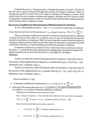
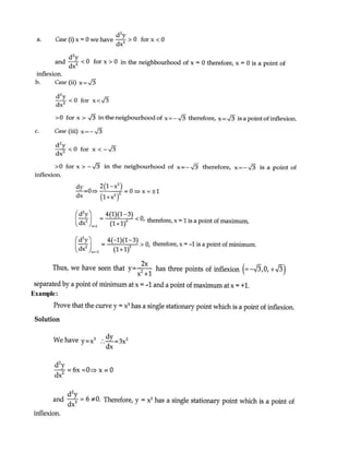
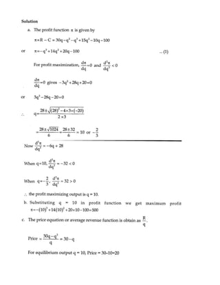
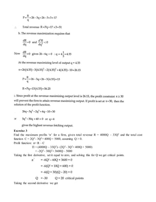
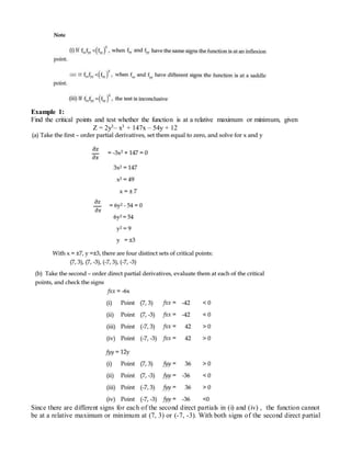
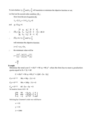
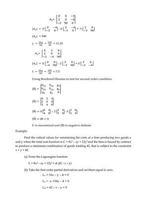
27. Constrained Optimization [With Lagrange Multipliers]
Differential calculus is also used to maximize or minimize a function subject to constant. Given a
function f(x, y) subject to a constraint g(x, y) = k, where k is a constant, a new function L can be formed
by setting the constraint equal to zero (that is, k – g(x, y) = 0), multiplying it by λ (that is, λ [k – g(x, y)]),
and adding the product to the original function:
L = f(x, y) + λ [k – g(x, y)]
Here L is the Largrangian function, λ is the Lagrange multiplier, f(x, y) is the original or objective
function, and g(x, y) is the constraint. Since the constraint is always set equal to zero, the product given
by λ[k – g(x, y)] also equals zero, and the addition of term does not change the value of the objective
function. Critical values x0, y0and λ0 at which the function is optimized, are found by taking the partial
derivatives of L with respect to all three independent variables (x, y and λ), setting them equal to zero,
and solving simultaneously.
If all the principal minors are negative, the bordered Hessian is positive definite, and a positive
definite Hessian always satisfies the sufficient condition for a relative minimum. If all principal
minors alternate consistently in sign from positive to negative, the bordered Hessian is negative
definite, and a negative definite Hessian always meets the sufficient condition for a relative maximum.

28. The HessianDeterminant
A Hessian determinant or simply a Hessian denoted as is a determinant composed of all the second
order partial derivatives. In the two variable case,
Example

29. Example
Higher Order Hessians

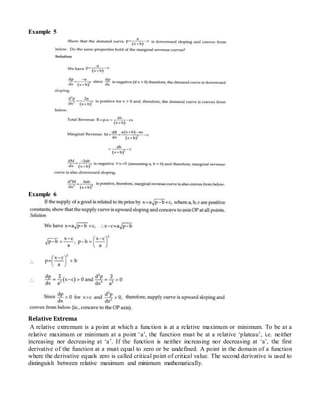
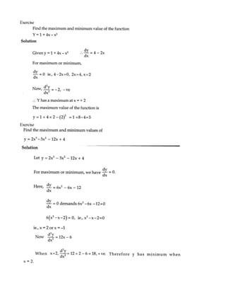
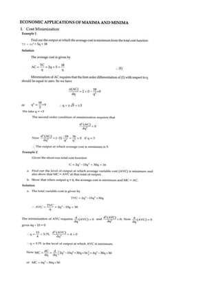
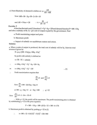
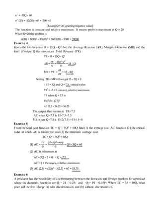
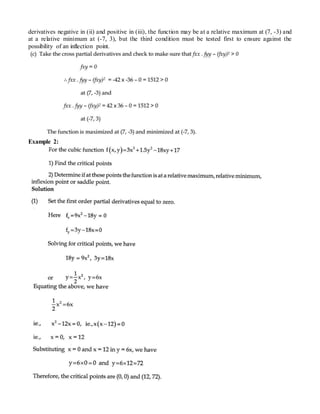
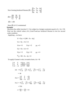
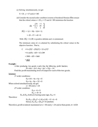
30. Example
BORDERED HESSIAN for Constrained Optimisation
Given a function, Z = f(x, y) subject to a constraint g(x, y) = k, where k is a constant, a new function
denoted as, say, F can be formed by
1) Setting the constraint equal to zero
2) Multiplying the constraint by language multiplier λ,
3) Adding the product to the original function.
That is, F = f(x, y) + λ [k- g (x, y)]
The first order conditions are found by taking partial derivatives of F with respect to all three
independent variables and setting them equal to zero. That is, Fx = 0, Fy = 0, Fλ = 0. The second order
conditions can be expressed in terms of bordered Hessian, denoted as

31. Example:
Optimize the function Z = 4x2+ 3xy + 6y2; Subject to the constraint x + y = 56

32. Significance of the Lagrange Multiplier
The Lagrange multiplier λ approximates the marginal impact on the objective function caused by a small
change in the constant of the constraint. With λ = 348 in the example presented above, for instance, a
one-unit increase (or decrease) in the constant of the constraint would cause z to increase (or decrease)
by approximately 348 units. Lagrange multipliers are often referred to as shadow prices. In utility
maximization subject to a budget constraint, for example, λ will estimate the marginal utility of an extra
unit of income.
Example

33. Example

34. Example

35. Example

37. Example:
A firm producing two goods x and y has the following profit function.
Π= 64x – 2x2+ 4xy – 4y2 + 32y – 14
Find the profit-maximizing level of output for each of the two goods.
Solution:
1st order conditions:
Πx= 64 – 4x + 4y = 0
Πy= 4x – 8y + 32 = 0
When solved simultaneously, we get
x = 40 and y = 24
2nd order condition:
Πxx= -4 < 0
Πyy = -8 < 0
Πxx & Πyy both are having same sign, Πxy= 4
Therefore
Πxx Πyy– (Πxy)2 = (-4) x (-8) – 42 = 6 > 0
Hence, Πxx Πyy– (Πxy)2> 0 satisfied.
Therefore, profit is indeed maximized at x = 40 and y = 24 and at that point, π= 1650