Software Techniques

1. ica imiza
ion
em
s
6. Classification Based on the Separability of the Functions
•^Optimization problems can be classified as separable and non-
separable
programmingproblems based on the separabilityof the objective and
constraint
functions.
• Separable Programming
Problem.
Definition A l”iinction J ïX) is ïillÔ tt) hU .$Jf1tli•i‹l›l‹ il it c:in bc «prcsscd :is ihc shir
of ii »inÿlc-i.mi.iblc t tiiietlt)n», ); ( i ; ). J_ t i_ ). . . . . J„ (.i„ J. th:il i».
.d
”‹v) ” ‹ ›.)

2. ica imiza
ion
em
s
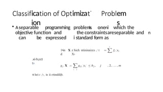
• separable programming problem one i which the
objective function and the constraintsareseparable and
can be expressed i standard form as
.xi‹h¡cct
t‹›
1•in
d
z hich ntininaizcs ,/ t
X›
i l
tt hci c /›, is ii ctinsliliJt.
If

3. 0 ^
€*-
0 >
'^
0 Ț
ir
»('^+'r+'‹)Oe’o
0«i‘S› ^ 'r os -» 'r oz I -* '•&
IX)**
fX)
£8
(
x
)
'
#
(X) '* oi iaa qns
ț

4. ica imiza ion
ems
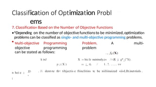
7. Classification Based on the Number of Objective Functions
•^Depending on the number of objectivefunctionsto be minimized,optimization
problems can be classified as single- and multi-objective programming problems.
• Multi-objective Programming Problem. A multi-
objective programming problem
can be stated as follows:
k inJ X ›‹ hic:lz naininaly.c« / t (
X j. g*_(”X).
p ; ( X ) < t). / l . ?. . . . . r›r
. Ji dent›te th< tibjectis e ftinclitins tc be niiIiinaized «ii«LIlt.inet›tiols .
n hei e .I
l
.$?-
-

5. imiza ems
sin
• MATLAB has severai tooiboxes each deveioped for the soiution of
probiems from a specific scientific area.
• The specific tooibox of interest for soiving optimization and related
problems is called the optimization toolbox.
• It contains a iibrary of programs or m-fiies, which can be used for
the solution of minimization, equations, least squares curve fitting,
and reiatedprobiems.

6. assic
a
imiza
ec
• The
various
techniques available for
the
ues
solution
of
different types
of
optimization problems.
• The classical methods of differential calculus can be used to find
the
unconstrained maxima and minima of a function of several variables. These
methods assume that the function is differentiable twice with respect to the
design variables and the derivatives are continuous.
• For problems with equality constraints, the Lagrange multiplier method can
be used.
• If the problem has inequality constraints, the Kuhn Tucker conditions can
be used to identify the optimum point.
• But these methods lead to a set of nonlinear simultaneous equations that may
be

7. assica imiza
• The classical methods of optimization are useful in finding the
optimum solution of continuous and differentiable functions.
• These methods are analytical and make use of the techniques of
differential calculus in locating the optimum points.
• Since some of the practical problems involve objective functions
that are not continuous and/or differentiable, the classical
optimization techniques have limited scope in practical applications.
• We will see the necessary and sufficient conditions in locating the
optimum solution of a single-variable function, a
multivariable function with no constraints, and a multivariable
function with equality and inequality constraints.

8. oca inimum
aximum
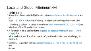
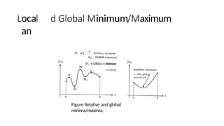
• A function of one variable f(x) is said to have a re/otive or local minimum at x =
x*
il f(x ) s f(x’+ h) for all sufficiently small positive and negative values of h.
• Similarly, a point x is called a relative or local maximumiff{x ) 2/{x + h) for
all values of h sufficiently close to zero.
• A function f(x) is said to have a global or absolute minimum at x il f(x
)1 f(x) for
all x, and not just for all x close to x*, in the domain over which f(x) is
defined.
• Similarly, a point x° will be a global maximum ol f (x) il f (x ) s: f (x) for all x in
the
domain.

9. oca
an
inimum aximum
A; ,•^2 2
'
RcIatIv€t mi*ñIx)ma
A2 = Giobal maximum
£;,D) —- Relative
m‹nima
Ay
A 3
Reiative minimum
is aISo giobal
minimum
Figure Relative and global
minima/maxima.

10. imiza
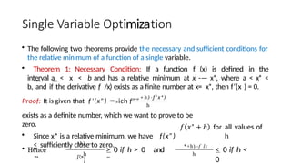
• The following two theorems provide the necessary and sufficient conditions for
the relative minimum of a function of a single variable.
• Theorem 1: Necessary Condition: If a function f (x) is defined in the
interval a < x < b and has a relative minimum at x -— x*, where a < x* <
b, and if the derivative f /x) exists as a finite number at x= x*, then f‘(x ) = 0.
Proof: It is given that f’(x”) hich f'””
+ h)-f(x*)
h
exists as a definite number, which we want to prove to be
zero.
• Since x* is a relative minimum, we have f(x”)
< sufficiently close to zero.
• Hence
"‘
h
+h) —
j’(x
)
> 0 if h > 0 and
"
*+h) -f lx
h
all values of
h
< 0 if h <
0

11. aria imiia
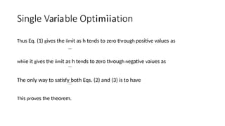
Thus Eq. (1) gives the iimit as h tends to zero through positive values as
whiie it gives the iimit as h tends to zero through negative vaiues as
The only way to satisfy both Eqs. (2) and (3) is to have
This proves the theorem.

12. imiza
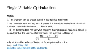
Notes:
1. This theorem can be proved even if x*is a relative maximum.
2.The theorem does not say what happens if a minimum or maximum occurs at
a point x* where the derivative fails to exist.
3.The theorem does not say what happens if a minimum or maximum occurs at
an endpoint of the interval of definition of the function. In this case
lim
h-•0
exists for positive values of h only or for negative values of h
only, and hence the
derivative is not defined at the endpoints.

13. imiza
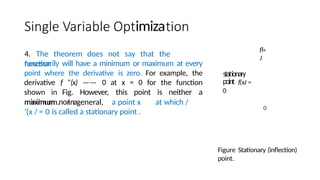
4. The theorem does not say that the
function
necessarily will have a minimum or maximum at every
point where the derivative is zero. For example, the
derivative f ”(x) —— 0 at x = 0 for the function
shown in Fig. However, this point is neither a
minimum nor a
stationary
point f(xJ =
0
maximum. In general, a point x at which /
’{x / = 0 is called a stationary point .
fl«
J
0
Figure Stationary (inflection)
point.

14. imiza
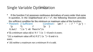
• If the function f (x) possesses continuous derivatives of every order that come
in question, in the neighborhood of x = x°, the following theorem provides
the sufficient condition for the minimum or maximum value of the function.
• Theorem 2 Sufficient Condition Let f
’(z *) f ”(x ')
0, but f ”) (x *) ¥0. Then//x*) is
•*(i) a minimum value ofj/x/ if f ”) (x ’) >0 and n is even;
*(ii) a maximum value off/x) if f(”) (x ”) < 0 and n is
even;
•’ (iii) neither a maximum nor a minimum if n is odd.
f ” 1
' (x ”)

15. aria imiia
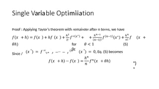
Proof : Appiying Tayior's theorem with remainder after n terms, we have
Since /
2!
for
0c
Eq. becomes
n!
*)
*

16. imiza
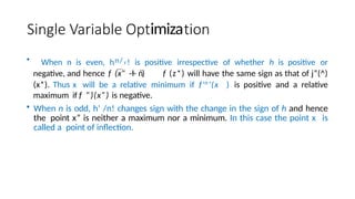
• When n is even, hn/‹! is positive irrespective of whether h is positive or
negative, and hence f (x” -ł- ń) f (z*) will have the same sign as that of j”(^)
(x*). Thus x will be a relative minimum if f'n
'(x ) is positive and a relative
maximum if f ”)(x”) is negative.
• When n is odd, h' /n! changes sign with the change in the sign of h and hence
the point x” is neither a maximum nor a minimum. In this case the point x is
called a point of inflection.