CADE

1. Advanced Optimization Theory
MED573
Multi Variable Optimization Algorithms
Dr. Aditi Sengupta
Department of Mechanical Engineering
IIT (ISM) Dhanbad
Email: aditi@iitism.ac.in
1

2. Introduction
2
• Methods used to optimize functions having multiple design variables.
• Some single variable optimization algorithms are used to perform
unidirectional search along desired direction.
• Broadly classified into two categories:
(i) Direct search methods
(ii) Gradient-based methods

3. • Optimality criteria differ from single-variable optimization.
• In multi-variable optimization, the gradient of a function is not a scalar quantity – it
is a vector quantity.
• Let us assume that the objective function is a function of N variables represented by
x1, x2, …, xN.
• The gradient at any point x(t) is represented by ∇𝑓𝑓 𝑥𝑥 𝑡𝑡
which is N-dimensional
vector given by
∇𝑓𝑓 𝑥𝑥 𝑡𝑡 =
𝜕𝜕𝜕𝜕
𝜕𝜕𝑥𝑥1
,
𝜕𝜕𝜕𝜕
𝜕𝜕𝑥𝑥2
, … ,
𝜕𝜕𝜕𝜕
𝜕𝜕𝑥𝑥𝑁𝑁
𝑇𝑇
at x(t)
3
Optimality Criteria

4. • The second-order derivatives form a matrix, ∇2𝑓𝑓(𝑥𝑥(𝑡𝑡)) known as Hessian matrix given by
∇2𝑓𝑓 𝑥𝑥 𝑡𝑡 =
𝜕𝜕2𝑓𝑓
𝜕𝜕𝑥𝑥1
2
𝜕𝜕2𝑓𝑓
𝜕𝜕𝑥𝑥1𝜕𝜕𝑥𝑥2
⋯
𝜕𝜕2𝑓𝑓
𝜕𝜕𝑥𝑥1𝜕𝜕𝑥𝑥𝑁𝑁
𝜕𝜕2𝑓𝑓
𝜕𝜕𝑥𝑥1𝜕𝜕𝑥𝑥2
𝜕𝜕2𝑓𝑓
𝜕𝜕𝑥𝑥2
2 ⋯
𝜕𝜕2𝑓𝑓
𝜕𝜕𝑥𝑥2𝜕𝜕𝑥𝑥𝑁𝑁
⋮ ⋮ ⋱ ⋮
𝜕𝜕2𝑓𝑓
𝜕𝜕𝑥𝑥𝑁𝑁𝜕𝜕𝑥𝑥1
𝜕𝜕2𝑓𝑓
𝜕𝜕𝑥𝑥𝑁𝑁𝜕𝜕𝑥𝑥2
⋯
𝜕𝜕2𝑓𝑓
𝜕𝜕𝑥𝑥𝑁𝑁
2
• Now that we have the derivatives, we are ready to define the optimality criteria.
• A point ̅
𝑥𝑥 is a stationary point if ∇𝑓𝑓 ̅
𝑥𝑥 = 0.
• The point is a minimum, a maximum or an inflection point if ∇2
𝑓𝑓 ̅
𝑥𝑥 is positive definite,
negative definite or otherwise.
4
Optimality Criteria

5. • The matrix ∇2𝑓𝑓(𝑥𝑥(𝑡𝑡)) is defined to be positive definite if for any point y in the
search space the quantity 𝑦𝑦𝑇𝑇∇2𝑓𝑓 𝑥𝑥 𝑡𝑡 𝑦𝑦 ≥ 0.
• The matrix ∇2𝑓𝑓(𝑥𝑥(𝑡𝑡)) is defined to be negative definite if for any point y in the
search space the quantity 𝑦𝑦𝑇𝑇
∇2
𝑓𝑓 𝑥𝑥 𝑡𝑡
𝑦𝑦 ≤ 0.
• If at some point y+ in the search space 𝑦𝑦+𝑇𝑇
∇2
𝑓𝑓 𝑥𝑥 𝑡𝑡
𝑦𝑦+
≥ 0 and for some other
point y-, 𝑦𝑦−𝑇𝑇∇2𝑓𝑓 𝑥𝑥 𝑡𝑡 𝑦𝑦− ≤ 0 then the matrix is neither positive definite nor
negative definite.
• Other test for positive definiteness – all eigenvalues are positive or if all principal
determinants are positive.
5
Optimality Criteria

6. • Successive unidirectional search techniques are used to find minimum along a search
direction.
• Unidirectional search is a one-dimensional search performed by comparing function
values only along a specified direction.
• Points that lie on a line (in N-dimensional space) passing through x(t) and oriented
along s(t) are considered in the search, expressed as
𝑥𝑥 𝛼𝛼 = 𝑥𝑥(𝑡𝑡)
+ 𝛼𝛼𝑠𝑠(𝑡𝑡)
Eq. (1)
where α is a scalar quantity.
6
Unidirectional Search

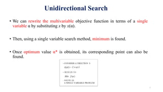
7. • We can rewrite the multivariable objective function in terms of a single
variable α by substituting x by x(α).
• Then, using a single variable search method, minimum is found.
• Once optimum value α* is obtained, its corresponding point can also be
found.
7
Unidirectional Search

8. Minimize f(x1, x2) = (x1 – 10)2 + (x2 – 10)2
The minimum lies at point (10, 10)T from the contour plot of
the function. Here, function value = 0.
Let the point of interest be x(t) = (2, 1)T and we are interested
in finding minimum and corresponding function value in
search direction s(t) = (2, 5)T.
From right-angled triangle shown in dotted line, the optimal
point obtained is x* = (6.207, 11.517)T.
Let us see if we can obtain the solution by performing
unidirectional search along s(t).
8
Unidirectional Search: Example

9. 9
Unidirectional Search: Example

10. We will use a bracketing algorithm to enclose optimum
point and then use a single-variable optimization method.
First, let us use bounding phase method. Assume initial
guess of x(0) = 0 and increment Δ = 0.5.
The bounds for α are obtained as (0.5, 3.5) with 6 function
evaluations. The bracketing points are then evaluated as
(3, 3.5)T and (9, 18.5)T.
Next, we use golden section search method to find
optimum point. Let us use a = 0.5 and b = 3.5. We obtain
α* = 2.103 as minimum.
Substituting α* = 2.1035, x(t) = (2, 1)T and s(t) = (2, 5)T in
Eq. (1), we obtain x* = (6.207, 11.517)T
10
Unidirectional Search: Example

11. • In single-variable optimization, there are only two search directions a point
can be modified – either in positive x-direction or negative x-direction.
• In multi-objective optimization, each variable can be modified either in
positive or negative directions leading to 2N ways of modification.
• One-variable-at-a-time algorithms cannot usually solve functions having
nonlinear interactions between design variables.
• Thus, we need to completely eliminate concept of search direction, and
instead manipulate a set of points to create a better set of points (eg.
Simplex search method).
11
Direct Search Methods

12. 12
Simplex Search Method
• For N variables, (N+1) points are to be used in the
initial simplex.
• To avoid a zero-volume hypercube for a N-variable
function, (N+1) points in the simplex should not lie
along the same line.
• At each iteration, the worst point in the simplex (xh)
is found first.
• Then, a new simplex is formed from the old simplex
by some fixed rules that “steer” the search away
from the worst point in the simplex.
Four situations may arise depending on function
values of the simplex.
1. First, the centroid (xc) of all but the worst point
is determined.
2. The worst point in the simplex is reflected about
xc and a new point xr is found.
3. If function value at xr is better than best point of
initial simplex, reflection is considered to have
taken simplex to a “good region” in search space.

13. 13
Simplex Search Method
4. An expansion along the line joining xc to xr is
performed, which is controlled by factor γ.
5. If function value at xr is worse than worst point
of initial simplex, reflection is considered to have
taken simplex to a “bad region” in search space.
6. Thus, a contraction along the line joining xc to xr is made, controlled by factor β.
7. Finally, if function value at xr is better than the worst point and worse than the next-to-worst
point in the simplex, contraction is made with β > 0.

14. 14
Simplex Search Method: Algorithm

15. 15
Simplex Search Method: Example

16. 16
Simplex Search Method: Example

17. 17
Simplex Search Method: Example

18. 18
Simplex Search Method: Example

19. 19
Simplex Search Method: Example

20. 20
Simplex Search Method: Example

21. 21
Simplex Search Method: Example

22. 22
Simplex Search Method: Example

23. 23
Simplex Search Method: Example

24. 24
Simplex Search Method: Example

25. 25
Simplex Search Method: Example

26. 26
Simplex Search Method: Example

27. First, we need to calculate the first and second-order derivatives for gradient-based methods. This is done using central
difference techniques as:
�
𝜕𝜕𝑓𝑓(𝑥𝑥)
𝜕𝜕𝑥𝑥𝑖𝑖 𝑥𝑥(𝑡𝑡)
= (f 𝑥𝑥𝑖𝑖
𝑡𝑡
+ ∆𝑥𝑥𝑖𝑖
𝑡𝑡
− f(𝑥𝑥𝑖𝑖
𝑡𝑡
− ∆𝑥𝑥𝑖𝑖
(𝑡𝑡)
))/(2∆𝑥𝑥𝑖𝑖
(𝑡𝑡)
)
�
𝜕𝜕2
𝑓𝑓(𝑥𝑥)
𝜕𝜕𝑥𝑥𝑖𝑖
2
𝑥𝑥(𝑡𝑡)
= (f 𝑥𝑥𝑖𝑖
𝑡𝑡
+ ∆𝑥𝑥𝑖𝑖
𝑡𝑡
− 2f(𝑥𝑥𝑖𝑖
𝑡𝑡
) + f(𝑥𝑥𝑖𝑖
𝑡𝑡
− ∆𝑥𝑥𝑖𝑖
(𝑡𝑡)
))/(∆𝑥𝑥𝑖𝑖
(𝑡𝑡)
)2
�
𝜕𝜕2
𝑓𝑓(𝑥𝑥)
𝜕𝜕𝑥𝑥𝑖𝑖 𝜕𝜕𝑥𝑥𝑗𝑗
𝑥𝑥(𝑡𝑡)
=
f 𝑥𝑥𝑖𝑖
𝑡𝑡
+ ∆𝑥𝑥𝑖𝑖
𝑡𝑡
, 𝑥𝑥𝑗𝑗
𝑡𝑡
+ ∆𝑥𝑥𝑗𝑗
𝑡𝑡
− f 𝑥𝑥𝑖𝑖
𝑡𝑡
+ ∆𝑥𝑥𝑖𝑖
𝑡𝑡
, 𝑥𝑥𝑗𝑗
𝑡𝑡
− ∆𝑥𝑥𝑗𝑗
𝑡𝑡
+ f 𝑥𝑥𝑖𝑖
𝑡𝑡
− ∆𝑥𝑥𝑖𝑖
𝑡𝑡
, 𝑥𝑥𝑗𝑗
𝑡𝑡
− ∆𝑥𝑥𝑗𝑗
𝑡𝑡
− f 𝑥𝑥𝑖𝑖
𝑡𝑡
− ∆𝑥𝑥𝑖𝑖
𝑡𝑡
, 𝑥𝑥𝑗𝑗
𝑡𝑡
+ ∆𝑥𝑥𝑗𝑗
𝑡𝑡
4∆𝑥𝑥𝑖𝑖
𝑡𝑡
∆𝑥𝑥𝑗𝑗
𝑡𝑡
For the complete first derivative vector of a N-variable function, 2N function evaluations are needed.
For the complete second derivative vector of a N-variable function, 3N function evaluations are needed.
For the complete mixed derivative vector of a N-variable function, 4N function evaluations are needed.
Thus, (2N2 +1) computations are needed for the Hessian matrix.
27
Gradient-Based Methods

28. • By definition, the first derivative represents direction
of the maximum increase of the function value.
• To get the minimum, we should be searching along
opposite to first derivative function.
28
Gradient-Based Methods
• Any search direction d(t) would have smaller function value than that at the current
point x(t).
• Thus, a search direction d(t) that satisfies the following relation is descent direction.

29. 29
Descent Direction
A search direction d(t) is a descent direction at point x(t) if the condition ∇𝑓𝑓 𝑥𝑥 𝑡𝑡 . 𝑑𝑑(𝑡𝑡) ≤ 0 is
satisfied in the vicinity of the point x(t).

30. 30
Cauchy’s Steepest Descent Method
• The search direction used in Cauchy’s method is the negative of the gradient at any
particular point x(k):
𝑠𝑠(𝑘𝑘)
= −∇𝑓𝑓(𝑥𝑥 𝑘𝑘
)
• Since this direction gives maximum descent in function values, it is known as steepest
descent method.
• At every iteration, derivative is calculated at current point and unidirectional search is
performed in direction which is negative to the derivative direction to find minimum
along that direction.
• The minimum point becomes current point and search is continued from this point.
• Algorithm continues till gradient converges to sufficiently small quantity.

31. 31
Cauchy’s Steepest Descent Method: Algorithm

32. 32
Cauchy’s Steepest Descent Method: Example
(See AOT2)

33. 33
Cauchy’s Steepest Descent Method: Example