Download to read offline


![• If we consider φ’’& φ’ are order of 1 objects in
magnitude .consider some limit , ether viscosity
going to be infinity or mass going to zero, remain
kind of on the order of one
• Consider f(φ) is order of 1
• φ’, φ”,f ~ order of 1
• Aim : neglect the acceleration term
• {r/(gT2)}φ” = {-br/(mgT)}φ’ + f (φ)
• We want scaling to choose T such that {br/mgT}~
order of 1
• Choose T={br/mg}
• Then (r/gT2)={r/[g(br/mg)2]} = (rm2g2/gb2r2)
• (m2g/b2r)<<1 (giving notation ϵ)
But (r/gT2)<<1](https://image.slidesharecdn.com/nonlineardynamics-230117083659-8a84c612/75/Non-Linear-Dynamics-Basics-and-Theory-29-2048.jpg)


![• P(N) = {BN2/A2+N2}
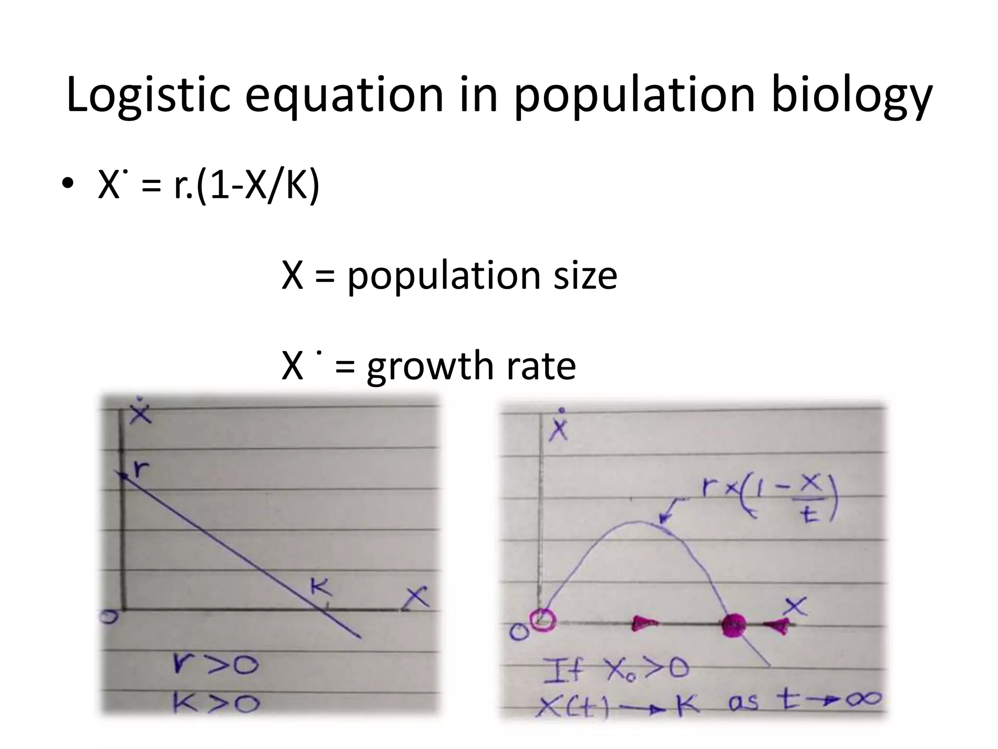
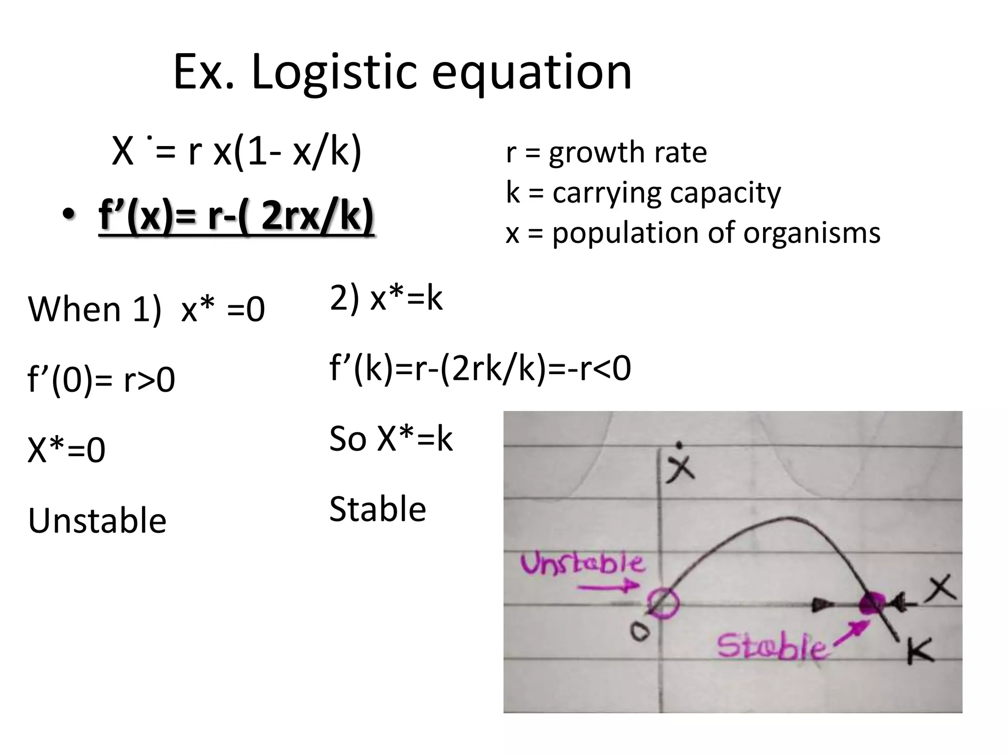
• X ˙= rx{1-(x/k)}
• Four parameters A,B,R,K
• Characteristics population sizes – A,K
• Choose scale of “N” to make the nonlinear P(N). Because
P(N)looking more nonlinear
• Let X= N/A
Eqn - N˙= RN {1-(N/K)} – P(N) becomes
• A(dx/dt) = RAX{1-(AX/K)}-{BA2X2/A2(1+X2)}
• (A/B) (dx/dt) = {R(AX/B){1-(AX/K)}} -{X2/(1+X2)}
• Let Ԏ= (Bt/A) (dimensionless time)
• X’ = rX[1-(X/K)] – (X2/1+X2)
r = growth rate
K= carrying capacity
X= population of organisms
N= AX
N˙= AX˙
Divide by B
We introduce hear dimensionless time
‘ = d/dԎ
Buckingham π theorem:
reduce 4 parameters to
2 dimensionless
parameters](https://image.slidesharecdn.com/nonlineardynamics-230117083659-8a84c612/75/Non-Linear-Dynamics-Basics-and-Theory-34-2048.jpg)


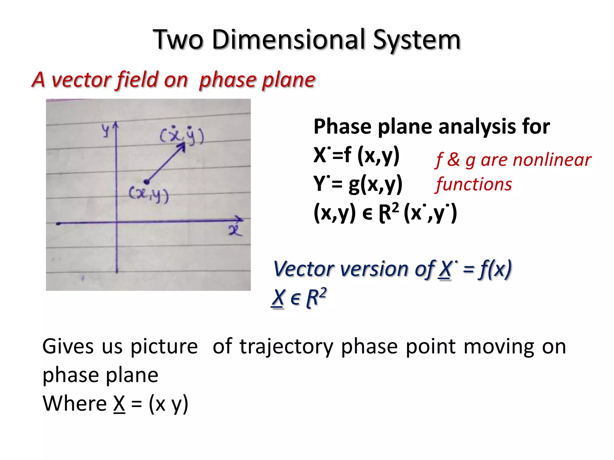
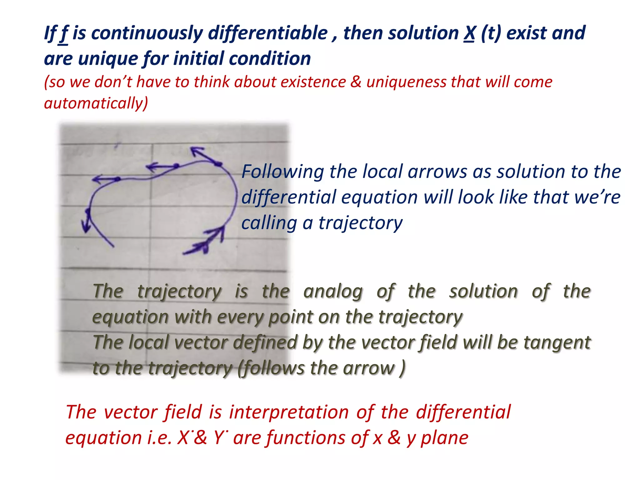
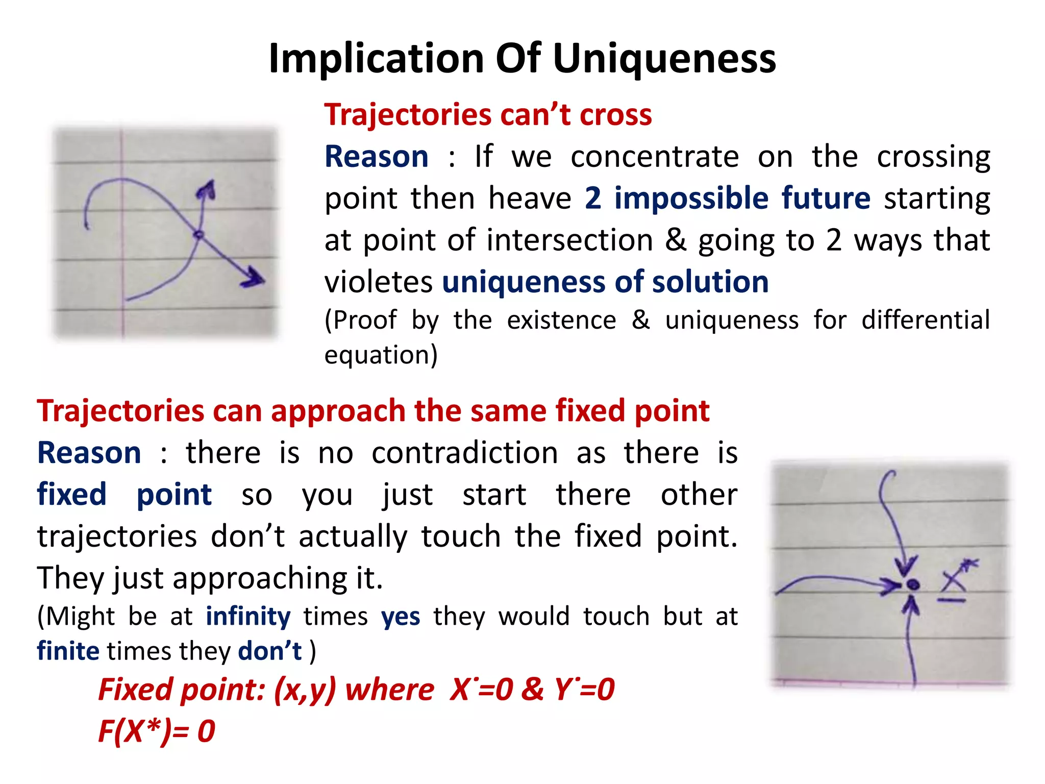
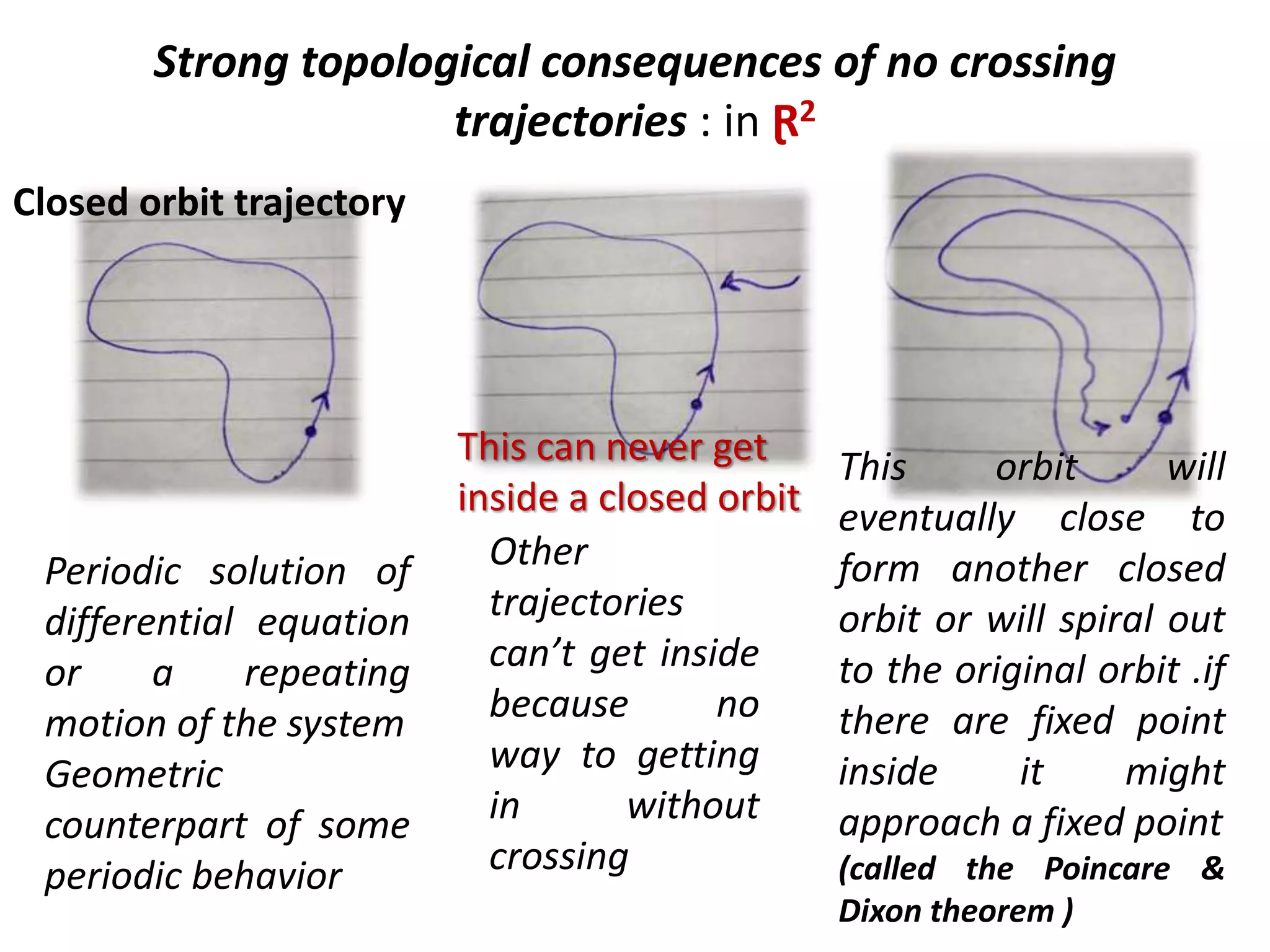

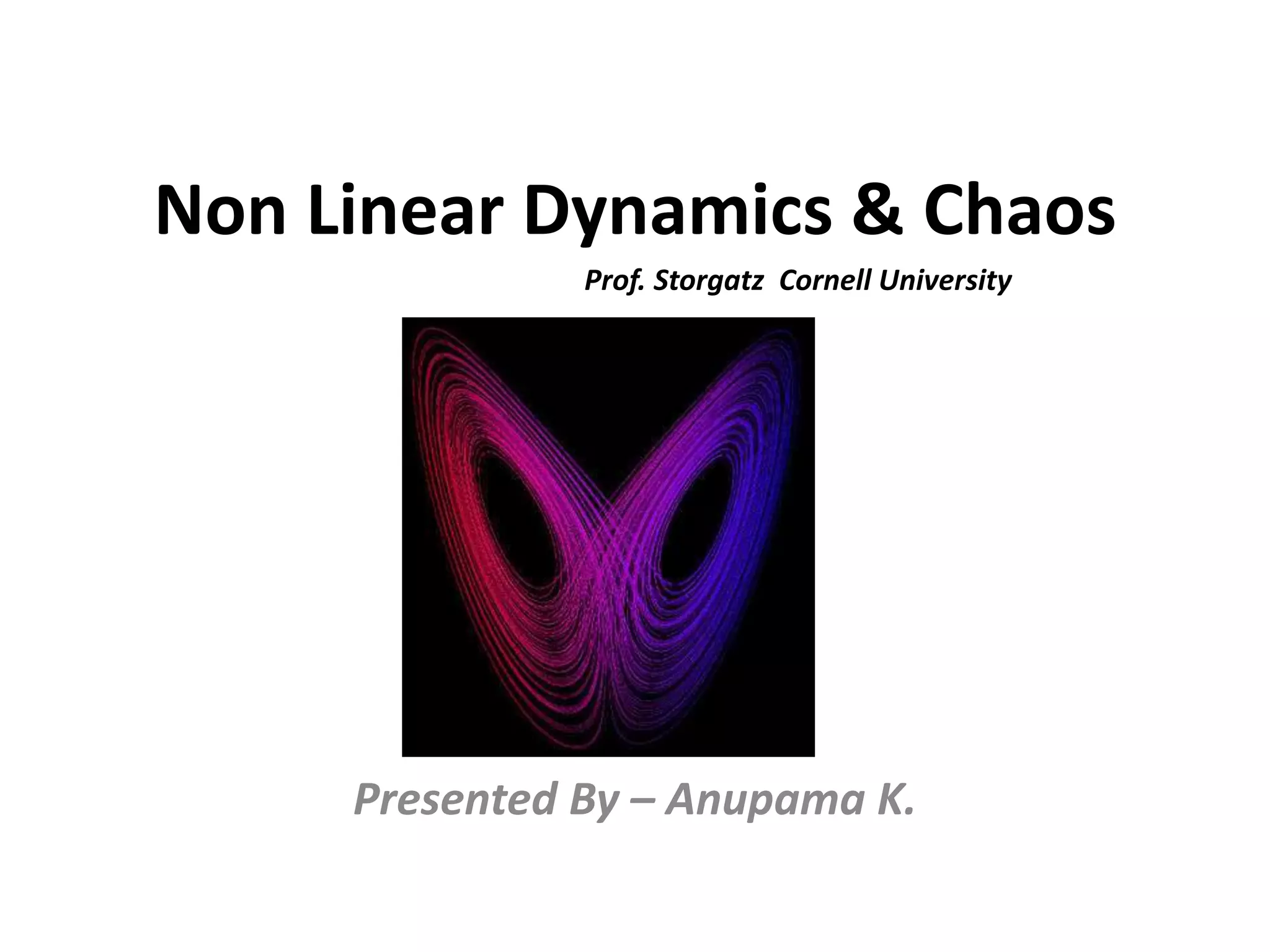
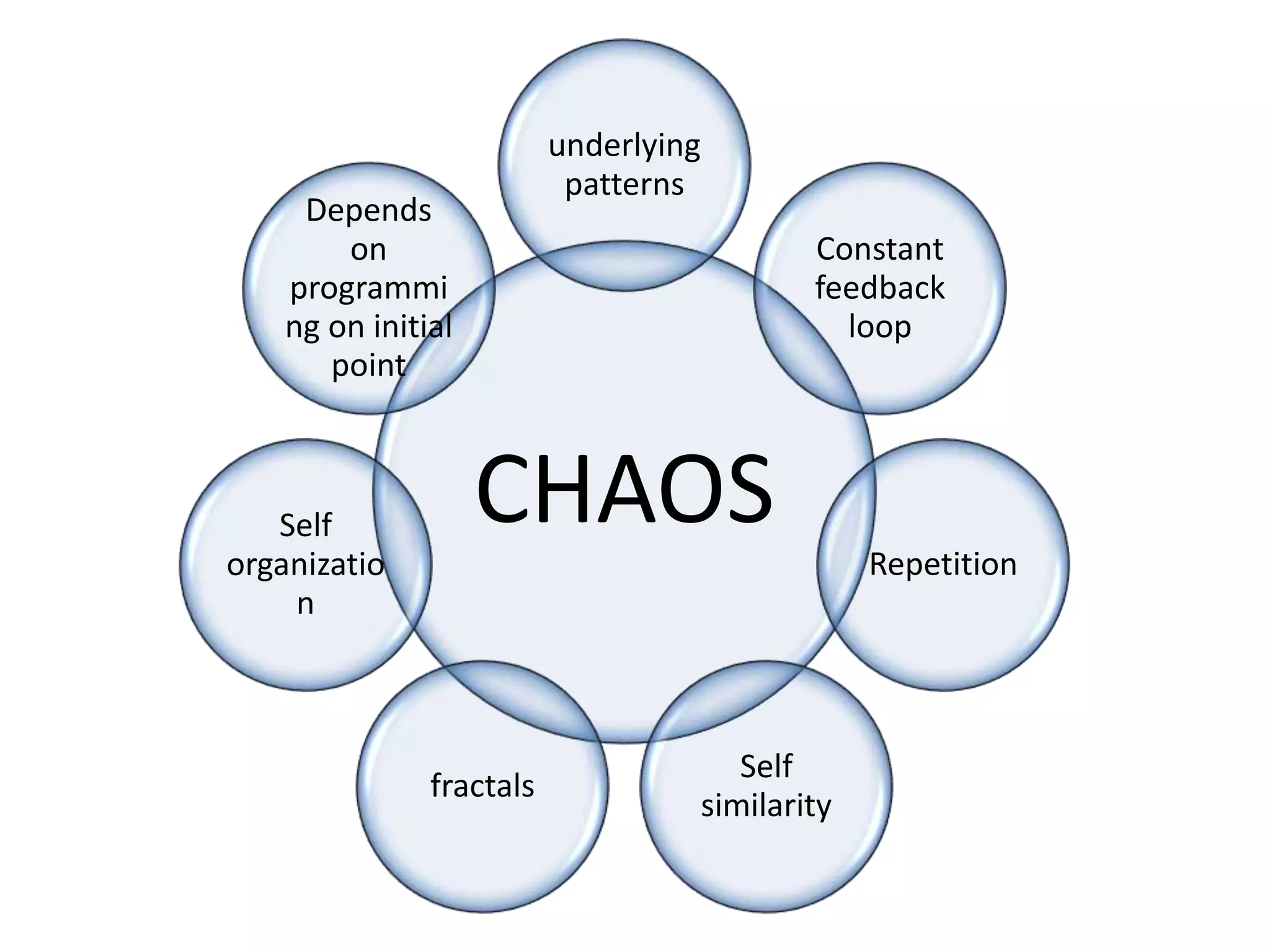
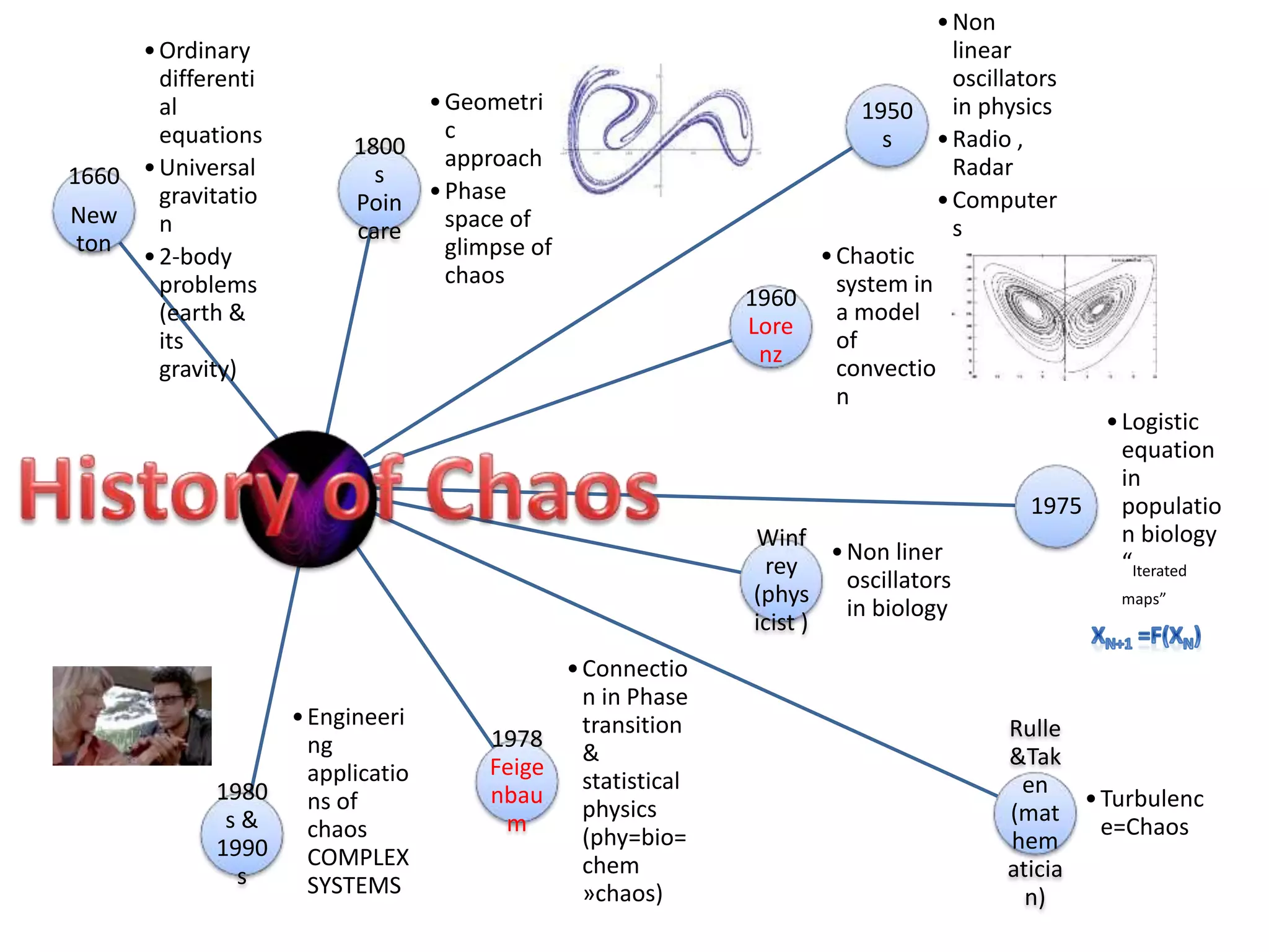
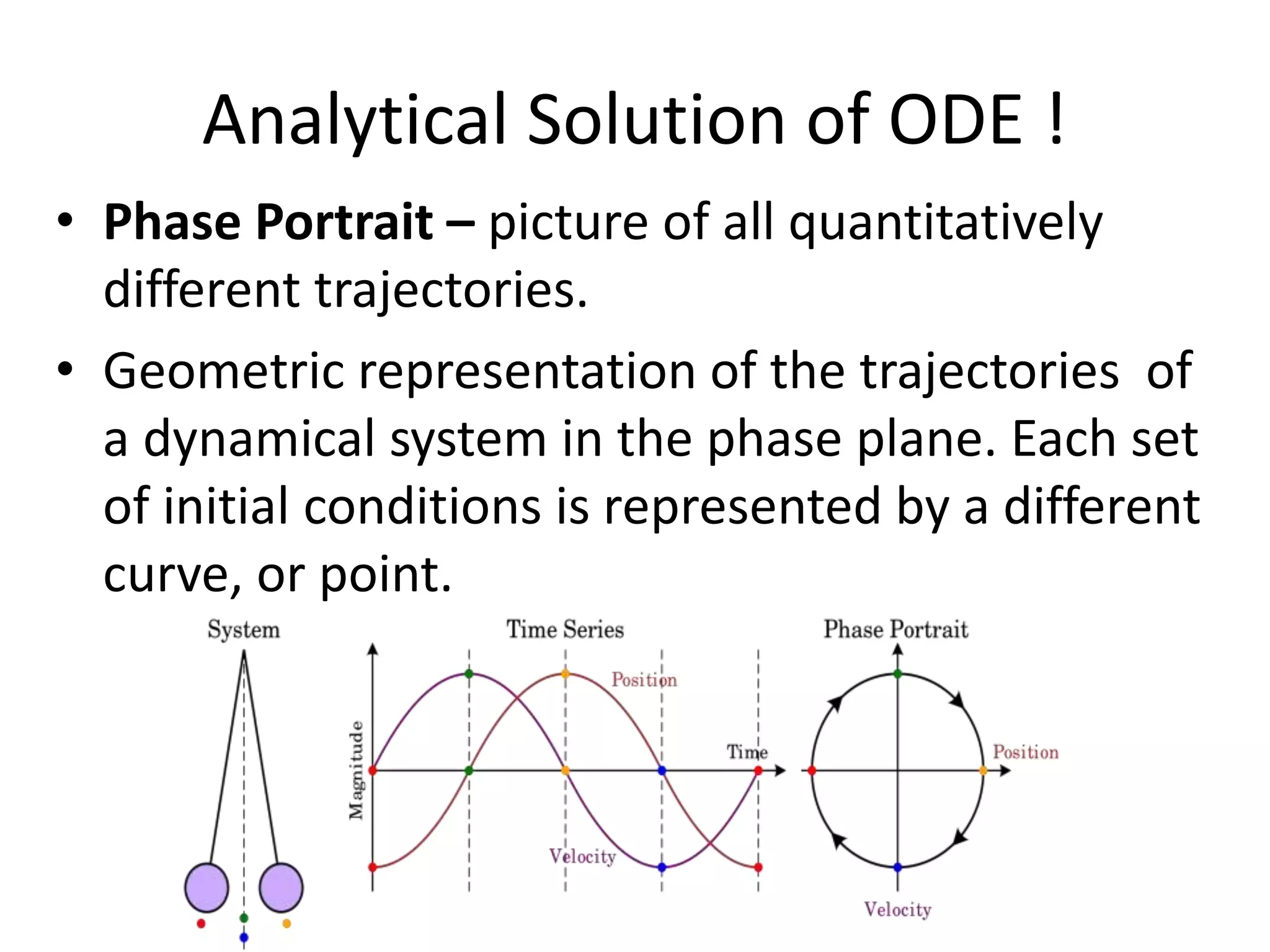
This document discusses nonlinear dynamics and chaos. It begins with an overview of key concepts in chaos like fractals, self-similarity, and dependence on initial conditions. It then provides a brief history of the field, covering contributions from Newton, Poincare, Lorentz, and others. The document proceeds to discuss logistic equations and bifurcations. It provides examples of fixed points, phase portraits, and bifurcation diagrams. It also covers modeling population dynamics and insect outbreaks using logistic growth equations.