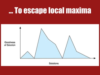
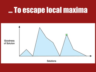
Simulated annealing is an algorithm for finding good solutions to optimization problems, such as the traveling salesman problem, where the goal is to find the shortest route between cities. It is inspired by annealing in metalworking, where heating and controlled cooling produces strong, defect-free metal. The algorithm starts with a random solution and finds neighboring solutions, accepting worse solutions with probability related to cost difference and iteration number, to avoid local optima. This allows big jumps early on, but the algorithm hones in on a local optimum over many iterations, usually finding a good enough solution. Parameters must be tuned correctly through trial and error. Overall, simulated annealing is considered effective for optimization problems.

1. Simulated Annealing
Katrina Ellison Geltman
Hacker School
February 20, 2014

2. What is
simulated annealing?

3. It’s an algorithm for finding a good solution to an
optimization problem

4. What’s an optimization
problem?

5. It’s the problem of finding the best solution from all
feasible solutions. (Wikipedia)

6. Canonical Example:
Traveling Salesman

7. Canonical Example:
Traveling Salesman
• The salesman needs to minimize the number of
miles he travels. An itinerary is better if it is
shorter.
• There are many feasible itineraries to choose
from. We are looking for the best one.

8. Simulated annealing solves this type of problem.

9. Why ‘annealing’?

10. • Simulated annealing is inspired by a
metalworking process called annealing.
• It uses the equation that describes changes in a
metal’s embodied energy during the annealing
process

11. How does it work?

12. The Process
!
!
!

13. The Process
• Generate a random solution!
• Assess its cost!
!
!
!

14. The Process
• Generate a random solution!
• Assess its cost!
• Find a neighboring solution!
• Assess its cost!
!

15. The Process
• Generate a random solution!
• Assess its cost!
• Find a neighboring solution!
• Assess its cost!
!• If cnew < cold: move!!
• If cnew > cold: maybe move

16. The Process
• Generate a random solution!
• Assess its cost!
• Find a neighboring solution!
• Assess its cost!
!• If cnew < cold: move!!
• If cnew > cold: maybe move
Why??

17. … To escape local maxima

18. … To escape local maxima

19. … To escape local maxima

20. … To escape local maxima

21. … To escape local maxima

22. The probability of accepting a worse solution
depends on:
> How much worse it is
> Which iteration you’re on

23. The probability of accepting a worse solution
depends on:
! ! > How much worse it is!
> Which iteration you’re on

24. The probability of accepting a worse solution
depends on:
! ! > How much worse it is!
> Which iteration you’re on
Typically
calculated using
Metropolis-
Hastings
algorithm

25. The probability of accepting a worse solution
depends on:
> How much worse it is
! ! > Which iteration you’re on

26. The probability of accepting a worse solution
depends on:
> How much worse it is
! ! > Which iteration you’re on
(later iteration = less likely)

27. The probability of accepting a worse solution
depends on:
> How much worse it is
! ! > Which iteration you’re on
Analogous to
temperature in the
physical
annealing
equation
(later iteration = less likely)

28. Big jumps to worse states happen early.
!
After many iterations, the algorithm hones in on a
local optimum.
!
So a good-enough solution is usually found.

29. The algorithm’s parameters must be tuned
correctly, which requires some guesswork.

30. But overall, simulated annealing is generally
considered a good choice for solving optimization
problems.

31. The End!