Mechanical Engineering Assignment Help

Mechanical Engineering
Assignment Help
For any help regarding Mechanical Engineering Assignment Help
visit :- https://www.matlabassignmentexperts.com/,
Email :- info@matlabassignmentexperts.com or
call us at :- +1 678 648 4277
matlabassignmentexperts.com

Problem 1 : Nonlinear parametric pendulum
The equation of motion governing an undamped simple pendulum is given by:
2
d 
dt2 0
2
 sin  0
0
where   g
L
is the natural frequency of the pendulum, g the acceleration due to gravity,
L the length of the pendulum and  the angle made with the vertical. Now, we can add a damping force to the equation by
including a term that is proportional to the velocity of the pendulum. The equation of motion now becomes:
d2
 
d 2
dt2
2  sin  0
dt 0
where  is the damping coefficient.
In this problem, we are interested in studying the nonlinear parametric pendulum, whose equation of motion is given by:
Problems
2
d  d
dt2
dt 0
2
 2   0
  
 
1 hcos 2 t sin  0
The above is a simple model for a child playing on a swing. The forcing term models the periodic pumping of the
child's legs at approximately twice the natural frequency of the swing. h is the amplitude of forcing. Let us see if we
can answer the following question in this problem: starting near the equilibrium point  ˙  0 , can the child get
the swing going by pumping his/her legs this way, or does he/she need a push ?

For this problem, choose 0 1. Unless otherwise specified, use   0.1. Also, remember that
 physically varies between 0 and 2 , and any value greater than 2 in the solution should be brought back to the
physical range using the function mod.
i) For the unforced and undamped pendulum ( h    0), find the time series  t vs. t
with the initial conditions:
a) 
˙0 0, 0 0.01
Show that the trajectory in a) is sinusoidal, whereas the trajectory in b) is not. This happens because, in part b),  is so
large thatsin   is not a good approximation, and hence nonlinear effects kick in. Also, show that the time period of
oscillations is dependent on the initial conditions for large  (and ˙), and is independent of the initial conditions for small
 (and ˙).
ii) The rest state  ˙ 0 of the pendulum is known to be unstable when
 2
 h 2
/16. V
erify the prediction of the critical value of
0
h necessary for sustained
oscillations of the pendulum. (Get the time series for two values of h , one that is just below and the other that is just
above the critical value of h given by the instability condition.)
iii) Plot the time series  t(for any initial condition) for h =1.50, 1.80, 2.00, 2.05, 2.062.
Calculate the time periods and comment on the pattern you observe. (Remember to let the initial transients die
away before you estimate the time period.)
b) 
˙0 0, 0 3

iv) The motion of the pendulum for h =2.2 is on a "strange attractor." An attractor (a set of points to which solutions get
attracted) is informally described as strange if the dynamics on the attractor are chaotic. When a system gets into the
chaotic regime, the behavior of the solution will seem random even though we have a deterministic system that governs
the motion of the pendulum. For h =2.2, plot the trajectory on a  ˙ plane, and observe the chaotic (random) nature of
the "strange attractor"! (Use any non-zero initial condition; you can also plot the time series of  or ˙ and observe that the
behavior is random and there is no clear time period in the signal.) Again, remember to let the initial transients die away
before you make your plots. Unpredictability is an essential feature of chaos. If a system is in the chaotic regime, it is
impossible to predict the exact position and velocity of the pendulum at a future time even if we are given the current
position and velocity with maximum accuracy. This property of unpredictability arises from what we call "sensitive
dependence on initial conditions." We may start the system at (0.1,0.1) and observe a specific trajectory; but, starting at
(0.1,0.10000001) may result in a completely different trajectory if the behavior is chaotic. Show that there is sensitive
dependence on initial conditions for h =2.2. (For showing sensitive dependence on initial conditions, consider two initial
conditions that are different only by a very small quantity (something like  = 0.001 radians should do the job), and
show that the solutions are very different after some time when plotted on top of each other.)
v) Finally, make a quick comparison of the time series of  for h =1.8, which is well
below the critical value for chaos, and h =2.2 when the system is chaotic. Use the same initial conditions for the two cases.
Problem 2 : The growth/decay of population of animal species
A popular model for the growth/decay of population of animal species is given by the logistic map. It takes into account the two
basic factors that contribute to the birth or death of any animal species:
a) Reproduction means the population will increase at a rate proportional to the current population. This can be stated as "the
population at a future time is proportional to the population at the current time," i.e.
xn1  xn

xn1
Where is the population at time n 1 given that the population at time n is xn .
The proportionality constant signifies the growth rate because of reproduction.
b) Starvation means the population will decrease at a rate proportional to the value obtained by taking the theoretical
"carrying capacity" of the environment less the current population. In a given environment, the presence of more
number of animals will result in more rapid consumption of the available resources, and this will result in more
likelihood of starvation. This can be written as
xn1  1 xn  xn1
Since xn and are normalized populations (actual population divided by the
maximum population possible), they cannot be greater than 1. 1 xn  is a measure of
how close the system is to the maximum carrying capacity of the environment. The proportionality constant
signifies the inverse of the death rate because of starvation.
Mathematically, the complete model that includes both the birth and the death processes can be written as:
xn1  rxn 1 xn 
where xn is a number between zero and one, and represents the population at year n ; hence
x0 represents the initial population (at year 0); r is a positive number, and represents a combined rate for reproduction
and starvation.
i) For values of r less than 1, show that, irrespective of the initial population, the population will eventually die.
r 1
,
ii) With r between 1 and 2, show that the population quickly stabilizes to the value r
independent of the initial population.
iii)What happens for values of r between 2 and 3 ?
iv) Play around with the value of r , and see if you can find a critical value above which the
n
solution no more converges to r 1
. Plotting x vs. n should reveal that the solution
r
never settles to a single value even for large n . Instead of converging to a single value,

the solution converges to a 2-period oscillation or a 4-period oscillation, or some
period oscillation as you increase r . At the first critical value of r , the solution will switch from settling to a single value to
settling to an oscillation between two values; similarly, at the second critical value of r , the solution will switch from settling to
an oscillation between two values to settling to an oscillation between four values; and so on. This is known as period-
doubling. As we can guess, for large enough r , the solution will
2k
converge to an oscillation between values, where k is large, and effectively, there
is no finite-period oscillation to which the system settles, and this is known as the "period-doubling route to chaos".
Show sample plots of xn Vs n for various values of r to confirm that period- doubling happens. Find the first four
values of r where period doubling occurs.
v) Create a rough map of the asymptotic values of xn for varying r . (What we are looking
for is the following: On the x-axis, you should plot r . On the y-axis should be the asymptotic values to which the
population converges for the corresponding value of r . The asymptotic values to which the population converges will be
either 1 or 2 or 4 or 8 or
2k
some in number depending on the value of r . You can do something like getting the
solution for a large number of iterations (say 50000) and plot the last 10000 values. If the solution converges to a single value,
we can expect the last 10000 values to be the same; if the solution converges to a 2-period oscillation, we can expect the last
10000 values to be switching between the two values of the 2-period oscillation, and so plotting the last 10000 values is
equivalent to plotting just the two values in the oscillation cycle; See the below figure which your rough map should look
like!).

vi) At r = 3.57 (approximately) is the onset of chaos, at the end of the period-doubling cascade. We can no longer see any
oscillations. Take r =3.7, and show that there is now sensitive dependence on initial conditions. (Slight variations in the
initial population yield dramatically different results over time, a prime characteristic of chaos. For more details on
unpredictability and sensitive dependence on initial conditions, see part iv) of the previous question.)
Problem 3 : Double-Well Potential System
External Force
F t F0 cost
x
g
x  0
The above figure shows a double well potential system. The double well is attached to a rigid framework and the particle
moves along the double well. As seen in the figure, the two wells are separated by a hump at x  0 has two stable states where
their potentials are minimal. So, it is called bistable system. The potential energy is proportional to the height of the
particle. Thedouble well potential can be expressed as V x  1
4
4
x  1
2
2
x . Suppose the double well is shaken
 
periodically by the external force from side to side. What happens to the motion of the damped particle? If the shaking is very
weak, the particle will go into one of the wells and stay near the bottom of the well, jiggling slightly. With strong shaking, the
particle trajectory will become larger. At this moment, we can guess that two types of particle motion exist: a small-amplitude,
low-energy oscillation about the bottom of a well, and a large-amplitude, high-energy oscillation where the particle goes back
and forth over the hump without settling down in one of the wells. Your task is to observe the particle motion under Stokes
type damping with coefficient  as a

function of initial conditions and the magnitude of external force. The motion equation of the particle along the double
well is given as follows: 3
0
ẋ
˙ ẋ  x  x  F cost
In this problem, the damping coefficient and the frequency of the external force are given:
  0.25 &  1.
i) Suppose that small external force F  0.18 is applied. Show that the motion of the particle depends on the initial
conditions. (You can choose different initial conditions, and calculate their trajectory, and compare together. 100-200
sec is enough to simulate the motion.) Confirm that all the trajectories of the particle are oscillatory and confined to
single well at the steady state. Is there any change of the period for different initial conditions?
ii) Suppose that large external force F  0.4 is applied. Compare the particle trajectories
for different initial conditions. Are they relevant? Irrelevant? Or chaotic? Describe what you observe (for the definition of
chaos, see problem 1).
iii)Now, we introduce the phase plane analysis. Phase plane is sometimes very useful to
analyze the nonlinear dynamic motions. Phase plane is defined as the plot of xt (x
axis) vs. x˙t(y axis), and you can observe dynamic behavior, independent of time.
Generate phase plane plot for different initial conditions you used in ii) (separate plots), and compare them together. (Use
simulation time of 1000-2000 sec to observe the behavior well.)
iv) From iii), you may recognize phase plane analysis is hard to interpret. At this time, another nonlinear dynamic analysis
tool is suggested, Poincaré section. It is obtained by plotting Vs for the same phase.
xt ẋt
obtain time values when they have same phase. For example, the phase of the external force at t=0, 2π/ω, 4π/ω,  are
same.). From a physical view point, we take “snapshot” of the system at the same phase in each driver cycle. Plot Poincaré
section for the initial conditions used in ii). (Plot the points, not line between two points in the figures. 10000-20000 sec
simulation time is enough to generate Poincaré section.) Is it better than phase plane analysis in terms of visualization?
Describe what you observe for different initial conditions.

v) In general, chaos still happens even when time goes to the infinity, but this system has different type of chaos: with two initial
conditions which are close together, their trajectories aren’t similar even in the transient response. However, either trajectory
eventually goes to a steady state, depending on particle’s transient behavior. It is called transient chaos, and chaos happens
only in the transient response. To find suitable initial conditions, trial and error is used. Plot the trajectories of particle
separately for following initial conditions.
&
a. x0 0.177 ẋ 0 0.1
&
b. x0 0.176 ẋ 0 0.1
Use F  0.25 as the magnitude of external force and 500 sec as the simulation time. Describe what you observe by
comparing both trajectories.
vi) Now, you understand it can be very hard to predict the final state of this system depending on the initial condition.
Therefore, the sensitivity of initial condition is conveyed more vividly by the following graphical method.
a. Initial conditions for position and velocity should be 2.5  x0, ẋ0 2.5
b. Make a 101 x 101 color grids with each grid point representing the particle’s final state with the given initial
condition.
c. Calculate trajectory up to 500 second for each initial condition.
d. A red dot is placed in a corresponding grid point if the trajectory ends up in the right well.
e. Blue dot is placed in a corresponding grid point if the trajectory ends up in the left well.
Plot the color-coded grids for different initial conditions. Is it beautiful? (Hint: you plot the map with ‘imagesc’
function. This function requires matrix (grid) to be imaged in the figure. You define empty matrix for color coding. If color
is red in corresponding grid, matrix element has 1. Otherwise, it has -1.)

Problem 1 : Nonlinear parametric pendulum
i)
Nonlinear pendulum without damping and force can be simplified to
d2

dt2
2
sin  0 .
0
Simulation results with given two initial conditions (small angle motion and large angle motion) are compared (See
the below codes and figure). Runge-Kutta method is used, and simulation time is up to 50 second. For the increase
of simulation accuracy, maximum time step is set to 0.01 second. In the figure, for a), small angular one is
definitely sinusoidal, and its period (6.28 second) corresponds to the reciprocal of the natural frequency (1
rad/sec=1/2π Hz) of the pendulum, and it confirms the period is independent of the initial conditions, and sin   is
a good approximation since natural frequency is closely related to the period of the response with no force in linear
system. However, the period increases as the initial angle becomes larger. For b), the shape in the figure is not
sinusoidal any more though it’s still periodic. Therefore, the period is related to the initial condition for the initial
condition with large angle.
function P81_i
% Problem 8.1 : Nonlinear parametric pendulum
% Part i. Unforced and undamped pendulum
% Define some constants
omega0=1; % Natural frequency of the pendulum
% Define some parameters for using Runge-Kutta metod
Solutions

tspan=[0 50]; % Time span to be obtained
% Choose time step smaller than 0.01 sec optn=odeset('InitialStep',1e-
2,'MaxStep',1e-2);
% Simulation with small angle (theta(0)=0.01 radian) [T1,Y1]=ode45(@(t,x)
Npp(t,x,omega0),tspan,[0.01 0],optn);
% Simulation with large angle (theta(0)=3 radian) [T2,Y2]=ode45(@(t,x)
Npp(t,x,omega0),tspan,[3 0],optn);
% Plot and compare simulation results figure(1);
subplot(2,1,1); plot(T1,Y1(:,1),'r'); grid on; axis tight; xlabel('bfTime
(Sec)'); ylabel('bfAngle (Rad)'); title('bfTrajectory of the Pendulum with
theta(0)=0.01 & dtheta/dt(0)=0');
subplot(2,1,2); plot(T2,Y2(:,1),'b--'); grid on; axis tight; xlabel('bfTime
(Sec)'); ylabel('bfAngle (Rad)'); title('bfTrajectory of the Pendulum with
theta(0)=3 & dtheta/dt(0)=0');
end
function dx=Npp(t,x,omega0)
% Describe nonlinear parametric pendulum motion dx(1,1)=x(2);
dx(2,1)=-omega0^2*sin(x(1)); end

x 10
-3
10
Trajectory of the Pendulum with (0)=0.01 & d/dt(0)=0
5
0
-5
Angle
(Rad)
Angle
(Rad)
0 5 10 15 20 25 30 35 40
Time (Sec)
45 50
Trajectory of the Pendulum with (0)=3 & d/dt(0)=0
3
2
1
0
-1
-2 0 5 10 15 20 30
25
Time (Sec)
35 40 45 50
ii)
 2
 h 2
/16 ,
0
From the pendulum become stable when h  0.4with given
parameters in this problem. To verify the above prediction. Two h values are chosen: the ones
slightly smaller and larger the critical value h  0.4 ( h  0.39 and h  0.41 ) From the below figure
generated by the following m-codes, it is shown that the pendulum with h  0.39 becomes stable
since the angular position approaches to zero as time goes on (top plot), but the one with h  0.41
turns out to be unstable since the angular motion increases (bottom plot).
function P81_ii
% Part ii. Stability
omega0=1;
gamma=0.1;
% Natural frequency of the pendulum
% Damping coefficient

h=[0.39 0.41]; % Two amplitudes of forcing
% Define some parameters for using Runge-Kutta metod tspan=[0 500]; %
Time span to be obtained theta0=[0.01,0]; % Initial
conditions
% Choose time step smaller than 0.01 sec
optn=odeset('InitialStep',1e-2,'MaxStep',1e-2);
% Simulation with the amplitude of forcing smaller than critical value [T1,Y1]=ode45(@(t,x)
Npp(t,x,gamma,omega0,h(1)),tspan,theta0,optn);
% Simulation with the amplitude of forcing larger than critical value [T2,Y2]=ode45(@(t,x)
Npp(t,x,gamma,omega0,h(2)),tspan,theta0);
% Plot and compare simulation results figure(1);
subplot(2,1,1); plot(T1,Y1(:,1),'r'); grid on; axis tight; xlabel('bfTime (Sec)');
ylabel('bfAngle (Rad)'); title('bfTrajectory of the Pendulum with
gamma>(homega_0)^2/16 (h=0.39)');
subplot(2,1,2); plot(T2,Y2(:,1),'b--'); grid on; axis tight; xlabel('bfTime (Sec)');
ylabel('bfAngle (Rad)'); title('bfTrajectory of the Pendulum with
gamma<(homega_0)^2/16 (h=0.41)');
end
function dx=Npp(t,x,gamma,omega0,h)
dx(2,1)=-2*gamma*x(2)-omega0^2*(1+h*cos(2*omega0*t))*sin(x(1)); end

Angle
(Rad)
-3 Trajectory of the Pendulum with >(h0)2/16 (h=0.39)
x 10
10
5
0
-5 0 50 100 150 200 250 300 350 400 450 500
Time (Sec)
Trajectory of the Pendulum with <(h0
)2/16 (h=0.41)
Angle
(Rad)
0.02
0.01
0
-0.01
-0.02
0 50 100 150 200 250 300 350 400 450 500
Time (Sec)
iii)
With the below m-codes, 5 plots are represented with different h (But, same initial
conditions chosen arbitrarily). For plotting time series, all of them look so similar; the absolute values of slopes are
almost same. However, their differences are apparent when they are plotted in the phase space. At h  1.50 , a given
angular position has only one corresponding angular velocity (single curve), which means the period of the response is
2 second since 0 1 rad/sec . At h 1.80 , a given angular position has two
corresponding angular velocities (two curves). It means that the pendulum follows one of two trajectories first, and the
other next time. So, the pendulum rotates along the same trajectory with every other rotation. It confirms that the period
is now doubled, compared with the one at h  1.50 . (If you plot the response along the angular position from 2 to
2 , the trajectory is just single curve.) It is called ‘period doubling’, and its period is 4 second. Similar phenomenon
(period doubling) happens again at h  2.00 . (Its period is 8 second.) For h  2.05 , its period is close to 128
second or more since so many period doubling happen between h  2.00 and h  2.05. Between h  2.05 and

function P81_iii
% Part iii. Period doubling
omega0=1;
gamma=0.1;
h=[ 1.50 1.80 2.00 2.05 2.062]; % Five amplitudes of forcing
% Define some parameters for using Runge-Kutta metod tspan=[0 500]; %
Time span to be obtained theta0=[3,0]; % Initial conditions
% Choose time step smaller than 0.01 sec optn=odeset('InitialStep',1e-
2,'MaxStep',1e-2);
% Define plot color set
col={'r' ; 'b' ; 'g' ; 'm' ; 'c'};
for i=1:length(h)
% Simulation with different h
[T,Y]=ode45(@(t,x) Npp(t,x,gamma,omega0,h(i)),tspan,theta0,optn);
% Remove transient response (remove data smaller than 100 second) Y=Y(find(T>=100),:);
T=T(find(T>=100),:);
% Generate figure figure(i);
% Plot steady state response for given h subplot(2,1,1);
plot(T,Y(:,1),col{i}); grid on; axis tight;
xlabel('bfTime (second)'); ylabel('bfAngular Position theta (rad)');
h  2.62 , it period decreases down to about 32 second. It’s a general behavior of period change in the nonlinear
parametric pendulum.

title(['bfSteady State Response (t,theta) for given h='
num2str(h(i))]);
% Plot phase space for given h
% Use mod for the angular position (-pi<=theta<=+pi) subplot(2,1,2); p=plot(pi-
mod(Y(:,1),2*pi),Y(:,2),[col{i} '.']); set(p,'MarkerSize',2);
grid on; axis tight;
xlabel('bfAngular Position theta (rad)'); ylabel('bfAngular Velocity
dtheta/dt(rad/sec)'); title(['bfPhase Space (theta,dtheta/dt) for given h='
num2str(h(i))]); end
end

iv)
First figure contains the time responses of angular position and angular velocity of the pendulum, and second one represents
phase space of the pendulum’s response. (They are generated with following m-codes.) If the system is deterministic, the small
change of initial conditions makes the system response change a little. However, the system responses are very different even
with very similar initial conditions if system is chaotic. In the case of our nonlinear parametric pendulum case, the system is
either deterministic or chaotic, depending on its some parameters. In this problem, the amplitude of forcing
decides characteristics of pendulum’s response. Therefore, the pendulum with h  2.20
is chaotic and it shows sensitive dependence on initial conditions, based on figures below.
function P81_iv
% Part iv. Sensitive dependence on initial conditions

omega0=1;
gamma=0.1;
h=2.20;
% Amplitude of forcing
% Define some parameters for using Runge-Kutta metod
tspan=[0 500];
theta0=[1e-1,0];
dtheta0=[0,1e-8];
% Time span to be obtained
% Initial conditions
% Change of initial conditions
% Simulation with given initial condition
[T,Y]=ode45(@(t,x) Npp(t,x,gamma,omega0,h),tspan,theta0,optn);
% Simulation with given initial condition + delta
[Td,Yd]=ode45(@(t,x) Npp(t,x,gamma,omega0,h),tspan,theta0+dtheta0,optn);
% Generate figure figure(1);
% Plot steady state response for given h subplot(2,1,1);
plot(T,Y(:,1),'r-',Td,Yd(:,1),'b--');
grid on; axis tight; xlabel('bfTime
(second)');
ylabel('bfAngular Position theta (rad)'); title('bfSteady State
Response (t,theta)'); legend('bftheta_0','bftheta_0+deltatheta',
...
'Location','NorthWest');
subplot(2,1,2); plot(T,Y(:,2),'r-',Td,Yd(:,2),'b--');
(second)');
ylabel('bfAngular Velocity dtheta/dt (rad/sec)');
title('bfResponse (t,dtheta/dt) with different initial conditions');
legend('bftheta_0','bftheta_0+deltatheta', ...
'Location','SouthWest');

% Plot phase space
% Use mod for the angular position (-pi<=theta<=+pi) figure(2);
p=plot(pi-mod(Y(:,1),2*pi),Y(:,2),'ro', ...
pi-mod(Yd(:,1),2*pi),Yd(:,2),'bs'); set(p,'MarkerSize',1);
xlabel('bfAngular Position theta (rad)'); ylabel('bfAngular Velocity
dtheta/dt(rad/sec)'); title('bfPhase Space (theta,dtheta/dt)');
legend('bftheta_0','bftheta_0+deltatheta', ...
'Location','SouthWest');
end

v)
With the below m-codes, the comparisons with different h are shown. As you see plots, they seem to have similar response at the beginning.
However, the responses are quite
different as time goes on. For h 1.80 , its response becomes steady and predictable. (the
pendulum seems to rotate clockwise constantly) However, the response with h  2.20 is neither stabilized nor predictable. The pendulum rotates
counterclockwise constantly, and it suddenly changes the rotating direction. Therefore, h  2.20 makes pendulum’s response chaotic.
function P81_v
% Part v. Sensitive dependence on initial conditions
omega0=1;
gamma=0.1;

h=[1.80 2.20]; % Two amplitudes of forcing
% Define some parameters for using Runge-Kutta metod tspan=[0 500];
% Time span to be obtained theta0=[1e-1,0];
% Initial conditions
% Simulation with h=1.8
[T1,Y1]=ode45(@(t,x) Npp(t,x,gamma,omega0,h(1)),tspan,theta0,optn);
% Simulation with h=2.2
[T2,Y2]=ode45(@(t,x) Npp(t,x,gamma,omega0,h(2)),tspan,theta0,optn);
% Generate figure figure(1);
% Plot steady state response for given h plot(T1,Y1(:,1),'r-
',T2,Y2(:,1),'b--');
(second)');
ylabel('bfAngular Position theta (rad)'); title('bfResponse (t,theta) with
different h'); legend(['bfh=' num2str(h(1))],['bfh=' num2str(h(2))], ...
'Location','NorthWest');
end

Response (t,) with different h
0
200
0
-200
-400
-600
-800
400
h=1.8
h=2.2
50 100 150 200 250 300 350 400 450 500
Time (second)
Angular
Position

(rad)
Problem 2 : The growth/decay of population of animal species
i)
The following figures with m-codes described as below represent the normalized population with respect to year n with
different initial populations. Each subplot has
different r (0.1, 0.5, 0.7, and 0.9). As seen in the plots, for arbitrary r between 0 and 1, all the populations approach to zero as
time goes on regardless of their initial conditions.
function P82_i
% Problem 8.2 : The growth/decay of population of animal species
% i. Show x_n converges to zero when 0<r<1.
% Choose arbitrary r between 0 and 1 r=[0.1 0.5 0.7 0.9];
% Set initial population matrix x0=[0.1:0.1:0.9]';
% Set the population year nf=15;
% Define color setr col={'r' ; 'b' ; 'g' ; 'm'};
figure(1);
for j=1:length(r)

% Set the normalized population matrix
% row: different initial populatipon
% column: population year n xn=zeros(length(x0),nf);
% Calculate the quadratic recurrence equation x=x0;
for i=1:nf
xn(:,i)=r(j)*x.*(1-x); x=xn(:,i);
end
% Plot the normalized population for n subplot(2,2,j);
h=plot(0:nf,[x0 xn],[col{j} 's-']); set(h,'MarkerSize',6);
set(gca,'FontSize',18); grid on; axis tight;
xlabel('bfThe population at year (a.u.)'); ylabel('bfThe normalized
population x_n (a.u.)');
title(['bfThe Normalized Population for r=' num2str(r(j))]);
end end
The Normalized Population for r=0.1 The Normalized Population for r=0.5
0.8 0.8
0.6 0.6
0.4 0.4
0.2 0.2
0 15
5 10
The population at year (a.u.)
0 15
5 10
The Normalized Population for r=0.7 The Normalized Population for r=0.9
The
normalized
population
x
(a.u.)
The
normalized
population
x
(a.u.)
n
n
The
normalized
population
x
(a.u.)
The
normalized
population
x
(a.u.)
n
n
0.8 0.8
0.6 0.6
0.4 0.4
0.2 0.2
0 15
5 10
0 15
5 10

ii)
In the same way as i), each subplot has different r (1.3, 1.5, 1.7, and 1.9). with these r ’s, below plots show the
normalized population as time goes on. Unlike i), the normalized population don’t approach to zero any more. Following
output lists the final values which the populations approach to.
1. r=1.300000
the population approaches to 0.230754 2. r=1.500000
the population approaches to 0.473684
With given r , each final values are same to
r 1
. Therefore, the final values for
r r
between 1 and 2 converge to r 1
.
r
function P82_ii
% ii. Show x_n converges to (r-1)/r when 1<r<2.
% Choose arbitrary r between 1 and 2 r=[1.3 1.5 1.7 1.9];
% Define color setr col={'r' ; 'b' ; 'g' ; 'm'};

figure(1);
for j=1:length(r)
% column: population year n
xn=zeros(length(x0),nf);
for i=1:nf
xn(:,i)=r(j)*x.*(1-x); x=xn(:,i);
end
% Plot the normalized population for n subplot(2,2,j);
figure(1);
h=plot(0:nf,[x0 xn],[col{j} 's-']);
set(h,'MarkerSize',6);
set(gca,'FontSize',18); grid on; axis tight;
% Display final values which the population approaches to fprintf('%d.
r=%fn',j,r(j));
fprintf('the population approaches to %fn',mean(xn(:,end)));
end end

0.8
0 30
5 10 15 20 25
The Normalized Population for r=1.3
0 30
0.2
0.4
0.6
0.8
5 10 15 20 25
0.6
0.4
0.2
0 30
5 10 15 20 25
The
normalized
population
x
(a.u.)
The
normalized
population
x
(a.u.)
n
n
0 30
0.2
0.4
0.6
0.8
5 10 15 20 25
The
normalized
population
x
(a.u.)
The
normalized
population
x
(a.u.)
n
n
0.8
0.6
0.4
0.2
iii) What happens for values of r between 2 and 3 ?
function P82_iii
% iii. What happens to x_n when 2<r<3.
% make series of r between 2 and 3 r=2.10:0.10:2.90;
for j=1:length(r)
% column: population year n xn=zeros(length(x0),nf);
for i=1:nf
xn(:,i)=r(j)*x.*(1-x);

x=xn(:,i);
end xf(j)=mean(xn(:,end));
end
% Plot the normalized population for n figure(1);
% Generate series r1=[2:0.01:3];
xf1=(r1-1)./r1;
%
h=plot(r,xf,'rs',r1,xf1,'b-');
set(h,'MarkerSize',6,'LineWidth',2); set(gca,'Fontsize',15);
legend('bfFinal Value of Population','bf(r-1)/r', ...
'Location','SouthEast');
end
The Normalized Population for 2<r<3
2 3
2.2 2.4 2.6 2.8
0.5
0.66
0.64
0.62
0.6
0.58
0.56
0.54
0.52
n
The
normalized
population
x
(a.u.)
Final Value of Population (r-1)/r

iv)
Below m-codes generate four plots whenever period-doubling happens as r increases from 2.90
to 3.60. As seen in the figure, each normalized population converges to an 2k
oscillation between different values. Another figure shows how many values exists
in single oscillation with respect to r . In addition to figures, the following output for m- code below is shown.
at r=2.900000, number of population =1
at r=3.000000, number of population =2 at r=3.450000, number of
population =4 at r=3.545000, number of population =8 at
r=3.565000, number of population =16 at r=3.569000, number of
population =28 at r=3.570000, number of population =69
at r=3.571000, number of population =129
at r=3.572000, number of population =150 at r=3.573000, number of
population =174
……
……
The number of different final populations is displayed doubled as r increases (2-period oscillation at r =3.000, 4-period
oscillation at r =3.450, 8-period oscillation at r =3.455, and 16-period oscillation at r =3.565). When r is close to
3.57, period-doubling happens any more since the number of different final populations increases randomly (look like
chaotic), and no finite-period oscillation doesn’t seem to exist. Therefore, 3.000, 3.450, 3.455, and 3.565 are the first
four values of r where period doubling occurs.
function P82_iv
% iv. period-doubling

% make series of r between 2.90 and 3.60
% with step size of 0.001 r=2.90:0.001:3.60;
% Set initial population x0=0.5;
% Define number of different final populations
n=zeros(1,length(r));
% Counter for number of period doubling happening j=1;
% Define color setr col={'r' ; 'b' ; 'g' ;
'm'};
% define figure figure(1);
% Simulation with different r for i=1:length(r)
% get 10000 values of final population
% 1. Simulation up to 40000 secs
% 2. Collect populations for next 10000 secs
% as final population. xn=LogiEqn(r(i),x0);
% Discard numbers below 0.001 xf=fix(xn*1000);
% Extract unique populations xf=unique(xf);
% Count number of unique populations n(i)=length(xf);
if i>1
% if period-doubling happens, display r if n(i)~=n(i-1)
fprintf('at r=%f, number of population =%dn', ... r(i),n(i));
% if the first 4 period-dobling, plot n vs. xn if j<=4
subplot(2,2,j);

plot([40001:50000],xn,[col{j} '.']);
axis tight; grid on; set(gca,'FontSize',16);
xlabel('bfYear (n)'); ylabel('bfNormalized Population
(x_n)');
title(['Number of period-doubling =' num2str(n(i))]); j=j+1;
end
end
% For starting point, else
fprintf('at r=%f, number of population =%dn', ... r(i),n(i));
end
end
% Plot r vs. number of unique populations figure(2);
plot(r,n,'r-');
xlabel('bfThe combined rate for reproduction and starvation (a.u.)'); ylabel('bfNumber of
Unique normalized populations');
title('bfNumber of Uniqie normalized population for 2.9<=r<=3.6'); end
function y=LogiEqn(r,x)
% Calculate quadratic reccureance relations
% x_n+1=r*x_n
% Calculate population for first 40000 years for i=1:40000
xn=r*x.*(1-x); x=xn;
end
% Define variable to store population for next 10000 years
y=zeros(length(x),10000);

% Calculate population for next 10000 years
for i=1:10000 xn=r*x.*(1-x);
x=xn; y(:,i)=xn;
end end
2.9 3.6
Number of Uniqie normalized population for 2.9<=r<=3.6
350
300
250
200
150
100
50
3 3.1 3.2 3.3 3.4 3.5
The combined rate for reproduction and starvation (a.u.)
Number
of
Unique
normalized
populations

v)
Following m-codes are for creating a rough map, and the figure represent a rough map of the asymptotic values
of xn for varying r .
function P82_v
% v.Plot r vs. x_infinity for logistic equation
% define the series of r from 0.01 to 4 with time step of 0.01 r=0.01:0.01:4;
% Calculate x_n when n approach to the infinity. for i=1:length(r)
% Obtain x_n for different very large n y=LogiEqn(r(i),0.1);
% Prepare the plot x=r(i)*ones(length(y),1);
% Generate the plot x_infinity distribution for the given r plot(x,y,'r.'); hold
on;
end
hold off;
axis tight; grid on; set(gca,'FontSize',16);
xlabel('bfThe combined rate for reproduction and starvation (a.u.)'); ylabel('bfThe
normalized population x_n for nrightarrowinfty');
end
function y=LogiEqn(r,x0)
%
% x_n+1=r*x_n
%
for i=1:40000 xn=r*x0.*(1-x0);

x0=xn;
end y=zeros(length(x0),10000); for i=1:10000
xn=r*x0.*(1-x0); x0=xn; y(:,i)=xn;
end end
vi)
Even if there is no oscillation, the sensitive dependence on initial conditions doesn’t
0 0
happen when initial populations x  x  0.5105
are chosen at r  3.57 . However,
the output of population for very very small amount of difference between two initial
0 0
populations ( x  x  0.5105
) at r  3.7 is quite different, and it confirms that there
is sensitive dependence on initial conditions. The m-codes and graphs for those outputs are shown as below.
function P82_vi

% vi. sensitive dependence on initial conditions
% Set two r's given in problem r=[3.57 3.7];
% Set initial population x0=0.5;
% set small difference of initial population dx0=0.00001;
for i=1:length(r)
% calcuate population with x0-dx0 xn1=LogiEqn(r(i),x0-
dx0);
% calcuate population with x0-dx0
xn2=LogiEqn(r(i),x0+dx0);
% plot and compare the results with above initial populations figure(i);
plot(0:length(xn1),[x0;xn1],'r*',0:length(xn2),[x0;xn2],'bo'); d=axis(); d(3:4)=[0
1]; axis(d); grid on; set(gca,'FontSize',24);
title(['bfThe Normalized Population for r=' num2str(r(i)) '& x_0=' num2str(x0)]);
legend('bfx_0-Deltax_0','bfx_0+Deltax_0','Location','SouthEast');
end end
function xn=LogiEqn(r,x0)
%
% x_n+1=r*x_n
% nf=500;
xn=zeros(nf,1); x=x0;
for i=1:nf

xn(i)=r*x.*(1-x);
x=xn(i);
end end
The Normalized Population for r=3.57& x0=0.5
1
0.9
0.8
0.7
0.6
0.5
0.4
0.3
0.2
0.1
x0-x0
x0+x0
0
0 50 100 150 200 250 300 350 400 450 500
The Normalized Population for r=3.7& x0=0.5
1
0.9
0.8
0.7
0.6
0.5
0.4
0.3
0.2
0.1
x0-x0
x0+x0
0
0 50 100 150 200 250 300 350 400 450 500
Problem 8.3 : Double-Well Potential System
i)
Two different initial conditions are used to observe their response. All the m-codes and figures are shown as below.
First of all, there responses are quite different, depending on
The
normalized
population
x
(a.u.)
The
normalized
population
x
(a.u.)
n
n

initial conditions. Second, their steady state responses are oscillatory. Finally, even though particles with different
initial conditions stay in one of two wells, their periods are didn’t change.
function P83_i
% Problem 8.3 : Double-Well Potential System
% i. Initial Condition Sensitivity for Small External Force
% Define some parameters
x01=[-0.05 0]; % First initial condition x02=[-0.05 -0.05];
% Second initial condition F=0.18; % Amplitude
of external force
% Solve equation of motion with the first initial conditions
[T1,X1]=ode45(@(t,x)DoubleWell(t,x,F),[0,100],x01);
% Solve equation of motion with the second initial conditions
% Plot and compare above two time response plot(T1,X1(:,1),'r-
',T2,X2(:,1),'b--');
grid on; axis tight; set(gca,'FontSize',14);
xlabel('bfTime (second)');
ylabel('bfLateral Trajectory of Particle (a.u.)'); title('bfInitial Condition
Sensitivity for Small External Force F=0.18');
legend('bfx_0=-0.05&v_0=0','bfx_0=-0.05&v_0=-0.05'); end
function dx=DoubleWell(t,x,F)
% Describe euation of motion
% in the double-well potetial system dx(1,1)=x(2);
dx(2,1)=F*cos(t)-0.25*x(2)+x(1)-x(1)^3; end

0 20 80 100
Initial Condition Sensitivity for Small External Force F=0.18
1
0.5
0
-0.5
-1
40 60
Time (second)
x =-0.05&v =0
0 0
x =-0.05&v =-0.05
0 0
Lateral
Trajectory
of
Particle
(a.u.)
ii)
In the same way as i), we compare particle trajectories for different initial conditions. Their responses are quite
different finally, even though their transient responses are a little similar. They are not periodic any more, they are
irrelevant, and seem to be chaotic.
function P83_ii
% i. Initial Condition Sensitivity for Large External Force
x01=[-0.05 0]; % First initial condition x02=[-0.05 -0.05];
% Second initial condition F=0.40; % Amplitude
of external force
% Plot and compare above two time response plot(T1,X1(:,1),'r-
',T2,X2(:,1),'b--');

legend('bfx_0=-0.05&v_0=0','bfx_0=-0.05&v_0=-0.05'); end
dx(2,1)=F*cos(t)-0.25*x(2)+x(1)-x(1)^3; end
0 20 80 100
40 60
Time (second)
iii)
Time responses obtained in i) and ii) are converted into position and velocity of particle trajectories. Phase planes for
different F and initial conditions are shown, which are generated by following m-codes. For F  0.18 , they shows
periodicity in steady state, but phase planes with F  0.40 don’t seems to have periodicity, even if the responses
are independent of time. (See below Figures)
-0.5
-1
-1.5
1.5
1
0.5
0
Lateral
Trajectory
of
Particle
(a.u.)
x =-0.05&v =0
0 0
x =-0.05&v =-0.05
0 0

function P83_iii
% iii. Phase Plane for different initial conditions
% and the amplitude of external force
% First initial condition
% Second initial condition
% Amplitude of external force
x01=[-0.05 0];
x02=[-0.05 -0.05];
F=[0.18 0.40];
% Create figure
figure(1);
for i=1:length(F)
[T1,X1]=ode45(@(t,x)DoubleWell(t,x,F(i)),[0,200],x01);
% Plot phase plane for the first initial conditions subplot(2,2,i*2-1);
plot(X1(:,1),X1(:,2),'r-'); grid on; axis tight;
set(gca,'FontSize',14); xlabel('bfLateral Position
(a.u.)'); ylabel('bfLateral Velocity (a.u.)');
title(['bfPhase Plane with x_0=-0.05&v_0=0 for F=' num2str(F(i))]);
[T2,X2]=ode45(@(t,x)DoubleWell(t,x,F(i)),[0,200],x02);
% Plot phase plane for the second initial conditions subplot(2,2,i*2);
plot(X2(:,1),X2(:,2),'b--');
xlabel('bfLateral Position (a.u.)'); ylabel('bfLateral
Velocity (a.u.)');
title(['bfPhase Plane with x_0=-0.05&v_0=-0.05 for F=' num2str(F(i))]);
end end

dx(2,1)=F*cos(t)-0.25*x(2)+x(1)-x(1)^3; end
=-0.05&v =0 for F=0.18
Phase Plane with x0 0
=-0.05&v =-0.05 for F=0.18
0.4
0.3
0.2
0.4
0 1.2
0.2 0.4 0.6 0.8 1
Lateral Position (a.u.)
-0.6
-1.2 -1 -0.8 -0.6 -0.4 -0.2 0
=-0.05&v =0 for F=0.4
=-0.05&v =-0.05 for F=0.4
1 1
Lateral
Velocity
(a.u.)
Lateral
Velocity
(a.u.)
0.1
0
-0.1
-0.2
-0.3
Lateral
Velocity
(a.u.)
Lateral
Velocity
(a.u.)
0.2
0
-0.2
-0.4
0.5 0.5
0
-1 -1
-1.5 -1 -0.5 0 0.5 1 1.5 -1.5 -1 -0.5 0 0.5 1 1.5
0
-0.5
-0.5
Lateral Position (a.u.) Lateral Position (a.u.)
iv)
Sometimes, Poincare section is quite useful in nonlinear dynamics analysis. We choose phase which is identical to
the multiple of 2 in the phase of oscillating external force. For small external force ( F  0.18 ), Poincare section
have several points for both initial conditions, but the position of points in Poincare section are completely different,
depending on initial conditions. Therefore, the phases of responses are synchronized with those of external forces,
and they are also periodic, but the position and velocity of particles during the oscillation depend on initial
conditions. For large external force( F  0.40 ), Their shapes for different initial conditions in Poincare
section are almost identical, independent of initial condition, even though they didn’t show any similarities in both
time response and phase plane analysis. It means that the position and velocity pairs of the particle at the multiple of
period for external force are same, independent of their pair’s sequence. Therefore, it confirms that time responses in
ii) are not chaotic, and they are relevant each other.

function P83_iv
% iv. Poincare section for different initial conditions
% and the amplitude of external force
% First initial condition
% Second initial condition
% Amplitude of external force
x01=[-0.05 0];
x02=[-0.05 -0.05];
F=[0.18 0.40];
% Create figure
figure(1);
for i=1:length(F)
[T1,X1]=ode45(@(t,x)DoubleWell(t,x,F(i)),[0:2*pi:20000],x01);
% Plot phase plane for the first initial conditions subplot(2,2,i*2-
1); plot(X1(:,1),X1(:,2),'r.'); grid on; axis tight;
set(gca,'FontSize',14); xlabel('bfLateral Position
(a.u.)'); ylabel('bfLateral Velocity (a.u.)');
title(['bfPoincare Section with x_0=-0.05&v_0=0 for F=' num2str(F(i))]);
[T2,X2]=ode45(@(t,x)DoubleWell(t,x,F(i)),[0:2*pi:20000],x02);
% Plot phase plane for the second initial conditions subplot(2,2,i*2);
plot(X2(:,1),X2(:,2),'b.');
xlabel('bfLateral Position (a.u.)'); ylabel('bfLateral
Velocity (a.u.)');
title(['bfPoincare Section with x_0=-0.05&v_0=-0.05 for F=' num2str(F(i))]);
end end

dx(1,1)=x(2);
dx(2,1)=F*cos(t)-0.25*x(2)+x(1)-x(1)^3; end
=-0.05&v =0 for F=0.18
Poincare Section with x0 0
=-0.05&v =-0.05 for F=0.18
0.3
0.1
0.25
Lateral
Velocity
(a.u.)
0.05
0
-0.05
Lateral
Velocity
(a.u.)
0.2
0.15
0.1
0.05
0
-0.1
-0.05
-1.2
0 1.2
0.2 0.4 0.6 0.8 1
-1 -0.8 -0.6 -0.4 -0.2
=-0.05&v =0 for F=0.4
=-0.05&v =-0.05 for F=0.4
1 1
0.8 0.8
Lateral
Velocity
(a.u.)
0.6
0.4
0.2
0
Lateral
Velocity
(a.u.)
0.6
0.4
0.2
0
-0.2 -0.2
-0.4 -0.4
-1 -0.5 0 0.5 1 -1 -0.5 0 0.5 1
Lateral Position (a.u.) Lateral Position (a.u.)
v)
Very small different initial condition (position difference is only 0.001, whereas velocity is same) give completely
different response and final well where the particle stays at the end. At the beginning, their transient responses are
almost same since they have very similar initial condition, but one of their response ( x0  0.178 ) goes to another well
suddenly due to some nonlinearity. (See following figure.) m-codes is also provided as below.
function P83_v
% v. Large Initial Condition Sensitivity
x01=[0.177 0.1]; % Initial condition for i)
x02=[0.178 0.1]; % Initial condition for ii)

F=0.25; % Amplitude of external force
% Solve equation of motion with initial conditions for i)
% Solve equation of motion with initial conditions for ii)
% Plot and compare above two time response
plot(T1,X1(:,1),'r-',T2,X2(:,1),'b--');
legend('bfx_0=0.177&v_0=0.1','bfx_0=0.178&v_0=0.1'); end
dx(2,1)=F*cos(t)-0.25*x(2)+x(1)-x(1)^3; end
1
0.5
-0.5
-1
0
Lateral
Trajectory
of
Particle
(a.u.)
x =0.177&v =0.1
0 0
x =0.178&v =0.1
0 0
0 100 400 500
200 300
Time (second)

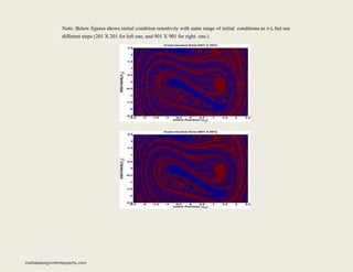
vi)
Following m-codes let you know how to generate color-coded grid, and display it as an image. See the below figure
shows the result of initial condition sensitivity for F  0.25 . As expected, the results of which well where the particle
stays eventually quite depend on the initial conditions in some range of initial condition.
function P83_vi
% vi. Plot the color-coded grids
% for different initial conditions.
% Define number of steps nx=50; ny=50;
% Define range of initial conditions mx=2.5; my=2.5;
% Generate full range of initial conditions x=[-nx:nx]/nx*mx;
y=[-ny:ny]/ny*my;
% Define Grid (101 X 101)
o=zeros(length(x),length(y));
% Calculate the final position o particle,
% depending on the initial conditions for i=1:length(x)
for j=1:length(y)
% Set initial condition x0=[x(i);y(j)];
% Calculate trajectory of particle
[T,X]=ode45(@DoubleWell,[0,500],x0);
% Determine which well the particle stays finally
o(i,j)=sign(X(end,1));
end
end
% Plot grid as an image with color code
% Swap row and column (Matrix transpose) o=o';

imagesc(o);
axis image; set(gca,'YDir','normal')
set(gca,'XTick',[1:10:101])
set(gca,'XTickLabel',[-2.5:0.5:2.5])
set(gca,'YTick',[1:10:101])
set(gca,'YTickLabel',[-2.5:0.5:2.5])
set(gca,'FontSize',20);
set(gca,'FontWeight','bold'); xlabel('bfInitial Position
(x_0)'); ylabel('bfInitial Velocity (v_0)');
title('bfInitial Condition Sensitivity in the Color-Coded Grid'); end
function dx=DoubleWell(t,x)
dx(2,1)=0.25*cos(t)-0.25*x(2)+x(1)-x(1)^3;
end
-2.5 -2 -1.5 -1 -0.5 0 0.5 1 1.5 2 2.5
Initial Position (x0)
Initial
Velocity
(v
0
)
Initial Condition Sensitivity in the Color-Coded Grid
2.5
2
1.5
1
0.5
0
-0.5
-1
-1.5
-2
-2.5

Note: Below figures shows initial condition sensitivity with same range of initial conditions as iv), but use
different steps (201 X 201 for left one, and 901 X 901 for right one.)

Mechanical Engineering Assignment Help

More Related Content

What's hot

Similar to Mechanical Engineering Assignment Help

More from Matlab Assignment Experts

Recently uploaded

Mechanical Engineering Assignment Help