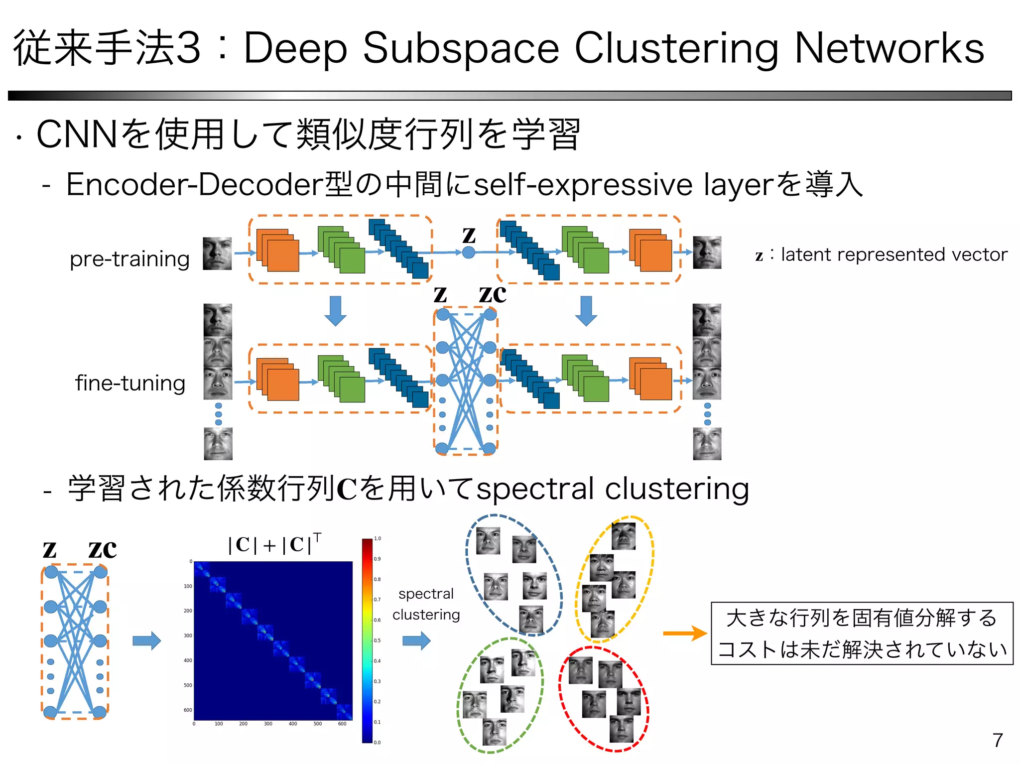
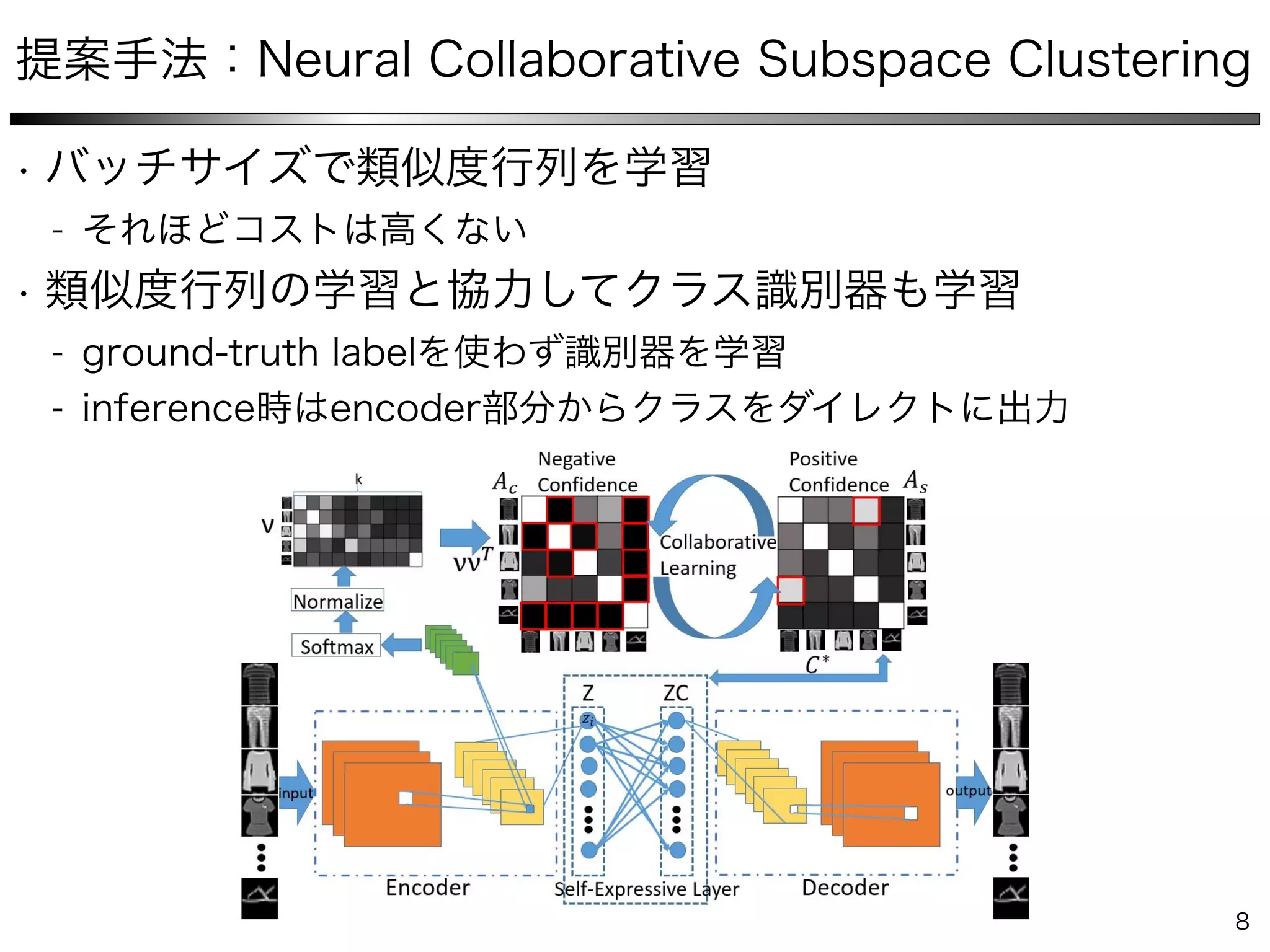
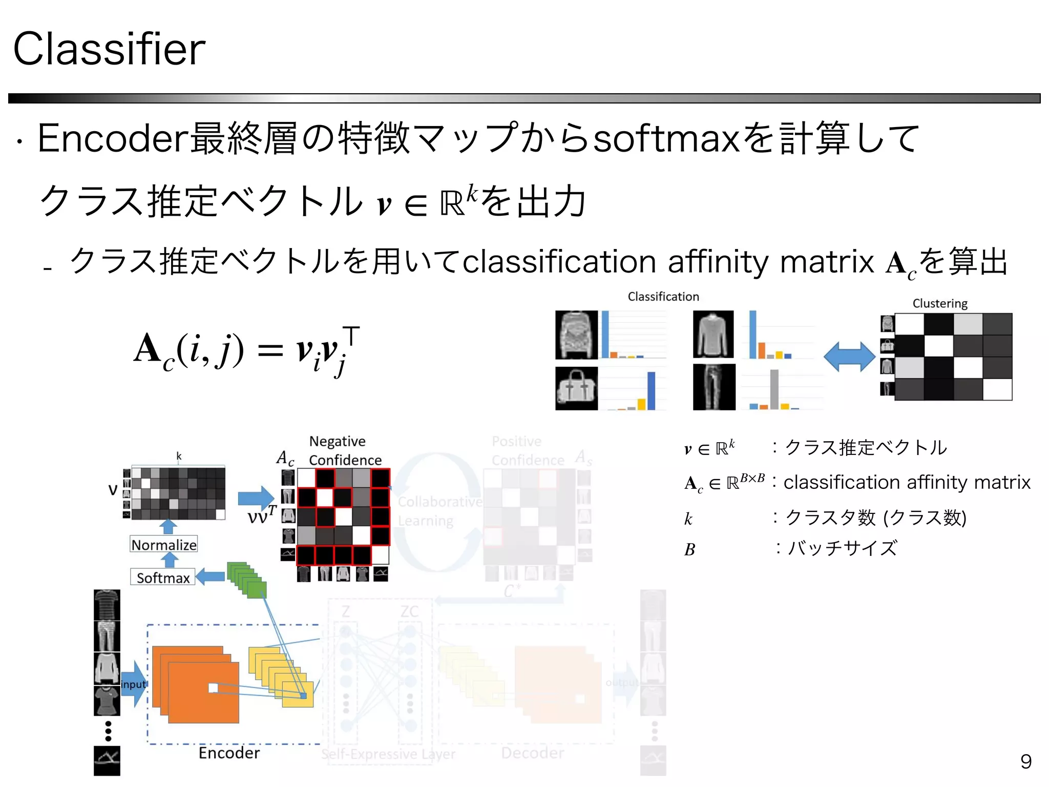
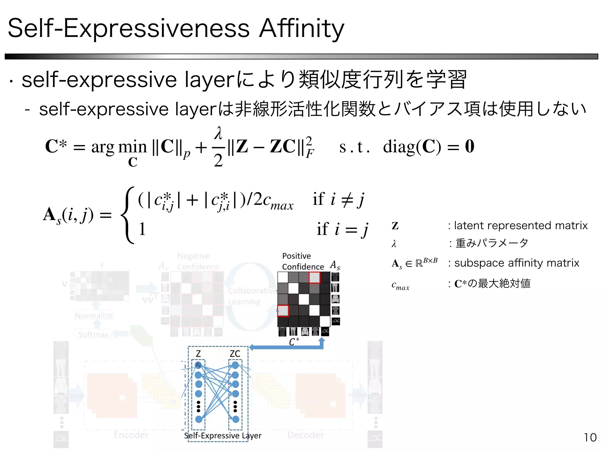
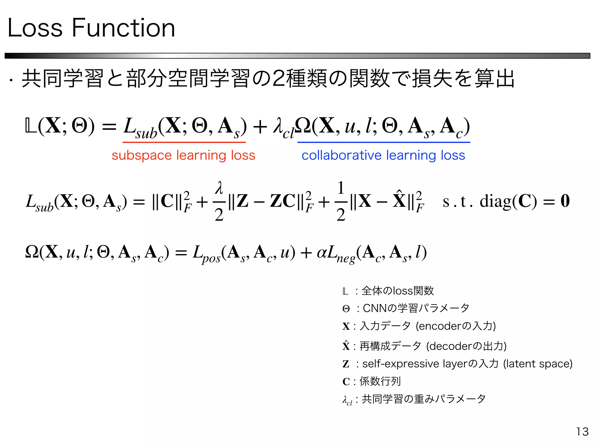
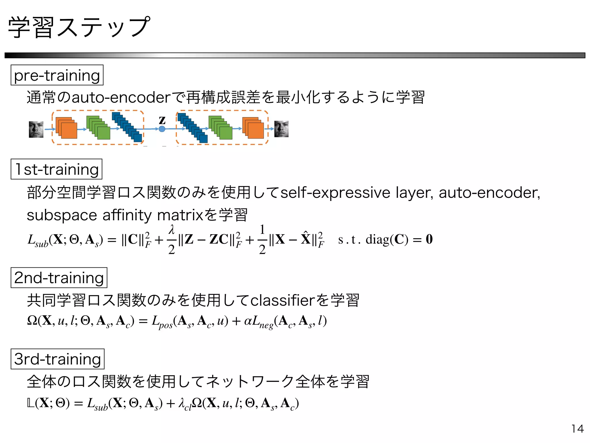
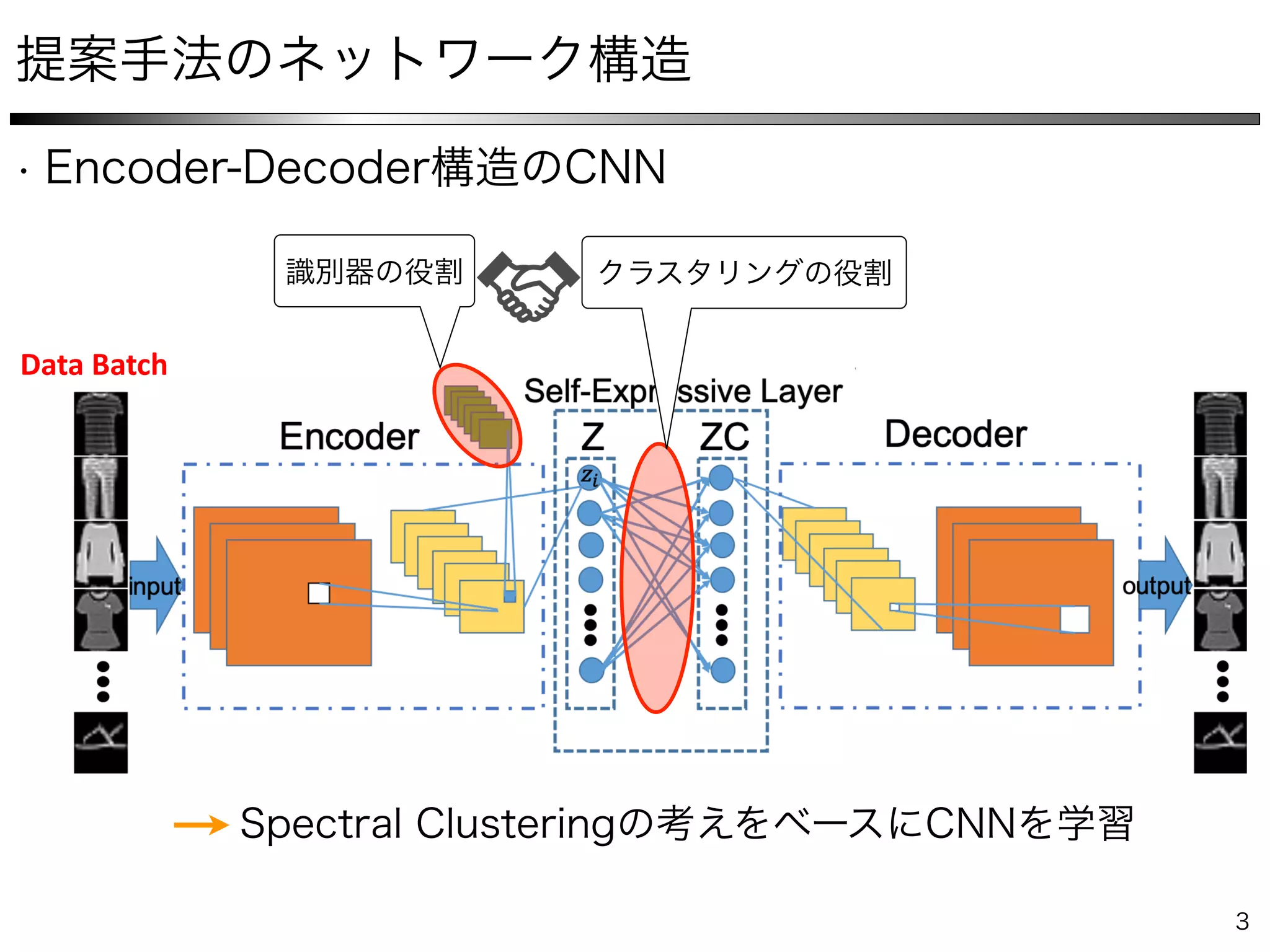
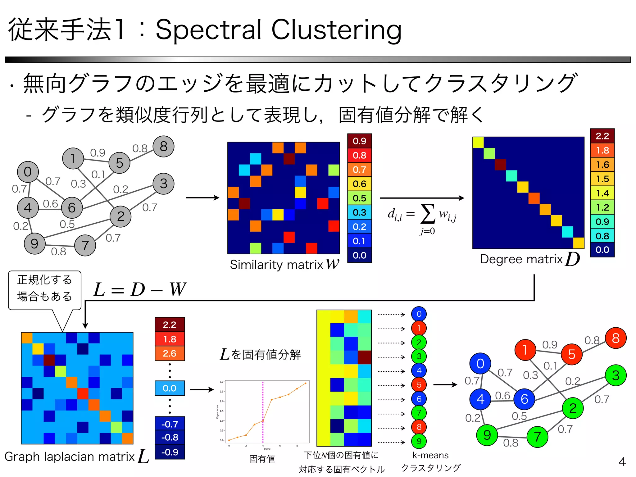
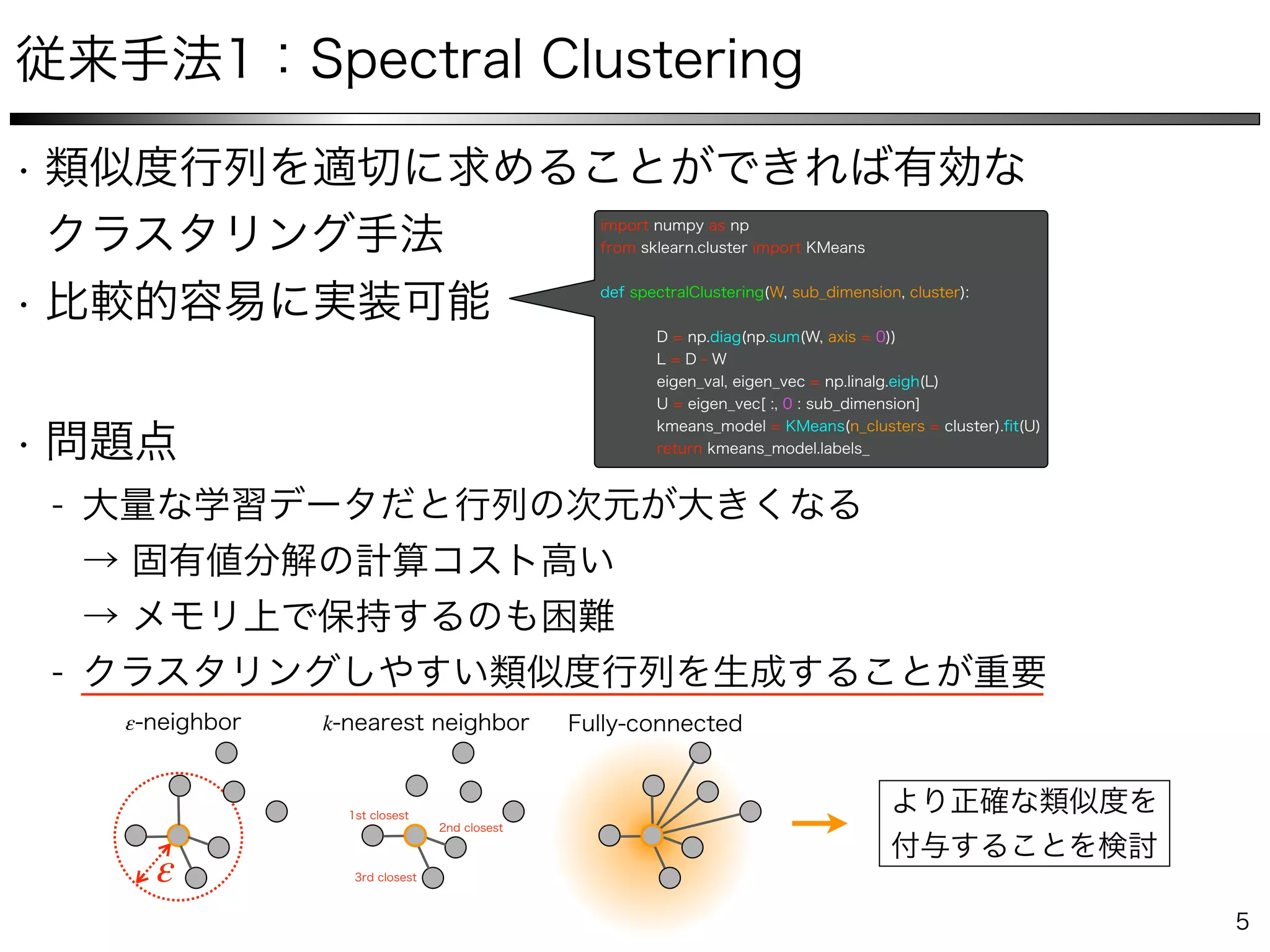
International Conference of Machine Learning (ICML), Long Beach, CA, June 10-15, 2019
Our Framework: Collaborative Learning
Data Batch
w D
di,i =
∑
j=0
wi,j
……
L
L = D − W
L
N


kε
ε


min
C
∥C∥p s . t . X = XC, diag(C) = 0 X ∈ ℝD×N
X = [x1, x2, ⋯, xN]
xi D
C ∈ ℝN×N 4
S1
S2
S3
yi
0 5 10 15 20 25 30
−0.05
0
0.05
0.1
q = ∞
0 5 10 15 20 25 30
−0.1
−0.05
0
0.05
0.1
0.15
q = 2
0 5 10 15 20 25 30
−0.2
0
0.2
0.4
q = 1
Fig. 3. Three subspaces in R3
with 10 data points in each subspace, ordered such that the fist and the last 10 points belong to S1 and
S3, respectively. The solution of the `q-minimization program in (3) for yi lying in S1 for q = 1, 2, 1 is shown. Note that as the value of q
decreases, the sparsity of the solution increases. For q = 1, the solution corresponds to choosing two other points lying in S1.
Different choices of q have different effects in the obtained
solution. Typically, by decreasing the value of q from infinity
toward zero, the sparsity of the solution increases, as shown in
Figure 3. The extreme case of q = 0 corresponds to the general
NP-hard problem [51] of finding the sparsest representation of
the given point, as the `0-norm counts the number of nonzero
elements of the solution. Since we are interested in efficiently
whose nonzero elements correspond to points from the same
subspace of the given data point. This provides an immediate
choice of the similarity matrix as W = |C| + |C|>
. In other
words, each node i connects itself to a node j by an edge whose
weight is equal to |cij|+|cji|. The reason for the symmetrization
is that, in general, a data point yi 2 S` can write itself as a
linear combination of some points including yj 2 S`. However,
4
S1
S2
S3
yi
0 5 10 15 20 25 30
−0.05
0
0.05
0.1
q = ∞
0 5 10 15 20 25 30
−0.1
−0.05
0
0.05
0.1
0.15
q = 2
0 5 10 15 20 25 30
−0.2
0
0.2
0.4
q = 1
Fig. 3. Three subspaces in R3
with 10 data points in each subspace, ordered such that the fist and the last 10 points belong to S1 and
S3, respectively. The solution of the `q-minimization program in (3) for yi lying in S1 for q = 1, 2, 1 is shown. Note that as the value of q
decreases, the sparsity of the solution increases. For q = 1, the solution corresponds to choosing two other points lying in S1.
Different choices of q have different effects in the obtained
solution. Typically, by decreasing the value of q from infinity
toward zero, the sparsity of the solution increases, as shown in
Figure 3. The extreme case of q = 0 corresponds to the general
NP-hard problem [51] of finding the sparsest representation of
the given point, as the `0-norm counts the number of nonzero
elements of the solution. Since we are interested in efficiently
whose nonzero elements correspond to points from the same
subspace of the given data point. This provides an immediate
choice of the similarity matrix as W = |C| + |C|>
. In other
words, each node i connects itself to a node j by an edge whose
weight is equal to |cij|+|cji|. The reason for the symmetrization
is that, in general, a data point yi 2 S` can write itself as a
linear combination of some points including yj 2 S`. However,
p = ∞ p = 1p = 2
{S1, S2, S3}
4
S1
S2
S3
yi
0 5 10 15 20 25 30
−0.05
0
0.05
0.1
q = ∞
0 5 10 15 20 25 30
−0.1
−0.05
0
0.05
0.1
0.15
q = 2
0 5 10 15 20 25 30
−0.2
0
0.2
0.4
q = 1
Fig. 3. Three subspaces in R3
with 10 data points in each subspace, ordered such that the fist and the last 10 points belong to S1 and
S3, respectively. The solution of the `q-minimization program in (3) for yi lying in S1 for q = 1, 2, 1 is shown. Note that as the value of q
decreases, the sparsity of the solution increases. For q = 1, the solution corresponds to choosing two other points lying in S1.
Different choices of q have different effects in the obtained
solution. Typically, by decreasing the value of q from infinity
toward zero, the sparsity of the solution increases, as shown in
Figure 3. The extreme case of q = 0 corresponds to the general
NP-hard problem [51] of finding the sparsest representation of
the given point, as the `0-norm counts the number of nonzero
whose nonzero elements correspond to points from the same
subspace of the given data point. This provides an immediate
choice of the similarity matrix as W = |C| + |C|>
. In other
words, each node i connects itself to a node j by an edge whose
weight is equal to |cij|+|cji|. The reason for the symmetrization
is that, in general, a data point yi 2 S` can write itself as a
xiS1
S2
S3
W = |C| + |C|⊤ ( wi,j = |ci,j | + |cj,i | ) W ∈ ℝN×N
C = C⊤
Figure 2: Deep Subspace Clustering Networks: As an example, we show a deep subspace clustering
network with three convolutional encoder layers, one self-expressive layer, and three deconvolutional
decoder layer. During training, we first pre-train the deep auto-encoder without the self-expressive
layer; we then fine-tune our entire network using this pre-trained model for initialization.
layer essentially lets us directly learn the affinity matrix via the network. Moreover, minimizing
kCkp simply translates to adding a regularizer to the weights of the self-expressive layer. In this
work, we consider two kinds of regularizations on C: (i) the `1 norm, resulting in a network denoted
by DSC-Net-L1; (ii) the `2 norm, resulting in a network denoted by DSC-Net-L2.
For notational consistency, let us denote the parameters of the self-expressive layer (which are just the
elements of C) as ⇥s. As can be seen from Figure 2, we then take the input to the decoder part of our
network to be the transformed latent representation Z⇥e
⇥s. This lets us re-write our loss function as
˜L(˜⇥) =
1
2
kX ˆX˜⇥k2
F + 1k⇥skp +
2
2
kZ⇥e
Z⇥e
⇥sk2
F s.t. (diag(⇥s) = 0) , (4)
where the network parameters ˜⇥ now consist of encoder parameters ⇥ , self-expressive layer
z
z zc
C
z zc |C| + |C|⊤
z
Neural Collaborative Subspace Clustering


v ∈ ℝk
Ac
Ac(i, j) = viv⊤
j
Neural Collaborative S
Figure 2. By normalizing the feature vectors after softmax func-
tion and computing their inner product, an affinity matrix can be
generated to encode the clustering information.
binary classifier by
Ac(i, j) = ⌫i⌫T
j , (1)
where ⌫i 2 Rk
is a k dimensional prediction vector after `2
normalization. Ideally, when ⌫i is one-hot, Ac is a binary
matrix encoding the confidence of data points belonging to
the same cluster. So if we supervise the classifier using Ac,
Neural Collaborative Subspace Clustering
v ∈ ℝk
Ac ∈ ℝB×B
k
B
Neural Collaborative Subspace Clustering
C* = arg min
C
∥C∥p +
λ
2
∥Z − ZC∥2
F s . t . diag(C) = 0
As(i, j) =
{
(|c*i,j | + |c*j,i |)/2cmax if i ≠ j
1 if i = j Z
λ
As ∈ ℝB×B
cmax C*

Ac As
Neural Collaborative Subspace Clustering
As
Ac
As Ac

Ac As
min
As,Ac
Ω(As, Ac, l, u) = Lpos(As, Ac, u) + αLneg(Ac, As, l)
Lpos(As, Ac, u) = H(Ms∥Ac) s . t . Ms = 𝔼(As > u)
International Conference of Machine Learning (ICML), Long Beach, CA, June 10-15, 2019
Collaborative Learning
• Subspace affinity is more confident of identifying samples from the
same class.
!"#$!%&'
Positive
Confidence
International Conference of Machine Learning (ICML), Long Beach, CA, June 10-15, 2019
Collaborative Learning
• Subspace affinity is more confident of identifying samples from the
same class.
!"#$!%&'
Positive
Confidence
Lneg(Ac, As, l) = H(Mc∥(1 − As)) s . t . Mc = 𝔼(Ac < l)
Collaborative Learning
• Subspace affinity is more confident of identifying samples from the
same class.
!"#$!%&'
Positive
Confidence
Collaborative Learning
• Subspace affinity is more confident of identifying samples from the
same class.
!"#$!%&'
Positive
Confidence
α
u, l
𝔼
H
H(p∥q) =
∑
j
pj log(qj)
𝕃(X; Θ) = Lsub(X; Θ, As) + λclΩ(X, u, l; Θ, As, Ac)
Lsub(X; Θ, As) = ∥C∥2
F +
λ
2
∥Z − ZC∥2
F +
1
2
∥X − ̂X∥2
F s . t . diag(C) = 0
Ω(X, u, l; Θ, As, Ac) = Lpos(As, Ac, u) + αLneg(Ac, As, l)
𝕃
Θ
X
̂X
Z
C
λcl
Figure 2: Deep Subspace Clustering Networks: As an example, we show a deep subspace clustering
network with three convolutional encoder layers, one self-expressive layer, and three deconvolutional
decoder layer. During training, we first pre-train the deep auto-encoder without the self-expressive
layer; we then fine-tune our entire network using this pre-trained model for initialization.
layer essentially lets us directly learn the affinity matrix via the network. Moreover, minimizing
kCkp simply translates to adding a regularizer to the weights of the self-expressive layer. In this
work, we consider two kinds of regularizations on C: (i) the `1 norm, resulting in a network denoted
by DSC-Net-L1; (ii) the `2 norm, resulting in a network denoted by DSC-Net-L2.
For notational consistency, let us denote the parameters of the self-expressive layer (which are just the
elements of C) as ⇥s. As can be seen from Figure 2, we then take the input to the decoder part of our
network to be the transformed latent representation Z⇥e
⇥s. This lets us re-write our loss function as
˜L(˜⇥) =
1
2
kX ˆX˜⇥k2
F + 1k⇥skp +
2
2
kZ⇥e
Z⇥e
⇥sk2
F s.t. (diag(⇥s) = 0) , (4)
where the network parameters ˜⇥ now consist of encoder parameters ⇥e, self-expressive layer
parameters ⇥s, and decoder parameters ⇥d, and where the reconstructed data ˆX is now a function of
{⇥e, ⇥s, ⇥d} rather than just {⇥e, ⇥d} in (3).
3.3 Network Architecture
z
Lsub(X; Θ, As) = ∥C∥2
F +
λ
2
∥Z − ZC∥2
F +
1
2
∥X − ̂X∥2
F s . t . diag(C) = 0
Ω(X, u, l; Θ, As, Ac) = Lpos(As, Ac, u) + αLneg(Ac, As, l)
𝕃(X; Θ) = Lsub(X; Θ, As) + λclΩ(X, u, l; Θ, As, Ac)
si = arg max
h
vi,h h = 1,2,⋯, k
si
vi
k
Neural Collaborative Subspace Clustering
Figure 1. The Neural Collaborative Subspace Clustering framework. The affinity matrix generated by self-expressive layer, As, and
ural Collaborative Subspace Clustering
images of size
ally for MNIST
entation among
ly our method
dle this type of
volutional auto-
ween the auto-
module. The
5 and channels
e classification
nal layers after
e convolutional
vector. For the
to 0.1 and 0.7
nd increase l to
5 mins to finish
GPU.
ACC(%) NMI(%) ARI(%)
CAE-KM 51.00 44.87 33.52
SAE-KM 81.29 73.78 67.00
KM 53.00 50.00 37.00
DEC 84.30 80.00 75.00
DCN 83.31 80.86 74.87
SSC-CAE 43.03 56.81 28.58
LRR-CAE 55.18 66.54 40.57
KSSC-CAE 58.48 67.74 49.38
DSC-Net 65.92 73.00 57.09
k-SCN 87.14 78.15 75.81
Ours 94.09 86.12 87.52
Table 1. Clustering results of different methods on MNIST. For
all quantitative metrics, the larger the better. The best results are
shown in bold.
without batch normalization in the encoder, and with a sym-
metric structure in the decoder. As the complexity of dataset
Neural Collaborative Subspace Clustering
The data samples of the Fashion-Mnist Dataset
ACC(%) NMI(%) ARI(%)
SAE-KM 54.35 58.53 41.86
CAE-KM 39.84 39.80 25.93
KM 47.58 51.24 34.86
DEC 59.00 60.10 44.60
DCN 58.67 59.4 43.04
DAC 61.50 63.20 50.20
ClusterGAN 63.00 64.00 -
InfoGAN 61.00 59.00 44.20
SSC-CAE 35.87 18.10 13.46
LRR-CAE 34.48 25.41 10.33
KSSC-CAE 38.17 19.73 14.74
DSC-Net 60.62 61.71 48.20
k-SCN 63.78 62.04 48.04
Ours 72.14 68.60 59.17
Table 2. Clustering results of different methods on Fashion-MNIST.
For all quantity metrics, the larger the better. The best results are
shown in bold.
ACC (%) NMI (%) ARI (%)
Neural Collaborative Subspace Clustering
Figure 3. The data samples of the Fashion-Mnist Dataset
ACC(%) NMI(%) ARI(%)
SAE-KM 54.35 58.53 41.86
CAE-KM 39.84 39.80 25.93
KM 47.58 51.24 34.86
DEC 59.00 60.10 44.60
DCN 58.67 59.4 43.04
DAC 61.50 63.20 50.20
ClusterGAN 63.00 64.00 -
InfoGAN 61.00 59.00 44.20
SSC-CAE 35.87 18.10 13.46
LRR-CAE 34.48 25.41 10.33
KSSC-CAE 38.17 19.73 14.74
DSC-Net 60.62 61.71 48.20
k-SCN 63.78 62.04 48.04
Ours 72.14 68.60 59.17
Table 2. Clustering results of different methods on Fashion-MNIST.
For all quantity metrics, the larger the better. The best results are
shown in bold.
ACC (%) NMI (%) ARI (%)
DEC 22.89 12.10 3.62
DCN 21.30 8.40 3.14
DAC 23.10 9.80 6.15
InfoGAN 19.76 8.15 3.79
Neural Collaborative Subspace Clustering
Figure 3. The data samples of the Fashion-Mnist Dataset
Figure 4. The visualization of our latent space through dimension
reduction by PCA.
ACC(%) NMI(%) ARI(%)
SAE-KM 54.35 58.53 41.86
CAE-KM 39.84 39.80 25.93
KM 47.58 51.24 34.86
DEC 59.00 60.10 44.60
DCN 58.67 59.4 43.04
DAC 61.50 63.20 50.20
ClusterGAN 63.00 64.00 -
InfoGAN 61.00 59.00 44.20
SSC-CAE 35.87 18.10 13.46
LRR-CAE 34.48 25.41 10.33
KSSC-CAE 38.17 19.73 14.74
DSC-Net 60.62 61.71 48.20
k-SCN 63.78 62.04 48.04
Ours 72.14 68.60 59.17
Table 2. Clustering results of different methods on Fashion-MNIST.
For all quantity metrics, the larger the better. The best results are
shown in bold.
ACC (%) NMI (%) ARI (%)
DEC 22.89 12.10 3.62
DCN 21.30 8.40 3.14
DAC 23.10 9.80 6.15
InfoGAN 19.76 8.15 3.79
SSC-CAE 12.66 0.73 0.19
LRR-CAE 22.35 17.36 4.04
KSSC-CAE 26.84 15.17 7.48
DSC-Net 26.87 14.56 8.75
k-SCN 22.91 16.57 7.27
data samples of the Fashion-Mnist Dataset
ualization of our latent space through dimension
.
shown Fig. 5.
or this dataset start from one layer convo-
with 10 channels, and follow with three
esidual blocks without batch normalization,
30 and 10 channels respectively.
the performance of all algorithms on this
KSSC-CAE 38.17 19.73 14.74
DSC-Net 60.62 61.71 48.20
k-SCN 63.78 62.04 48.04
Ours 72.14 68.60 59.17
Table 2. Clustering results of different methods on Fashion-MNIST
For all quantity metrics, the larger the better. The best results are
shown in bold.
ACC (%) NMI (%) ARI (%)
DEC 22.89 12.10 3.62
DCN 21.30 8.40 3.14
DAC 23.10 9.80 6.15
InfoGAN 19.76 8.15 3.79
SSC-CAE 12.66 0.73 0.19
LRR-CAE 22.35 17.36 4.04
KSSC-CAE 26.84 15.17 7.48
DSC-Net 26.87 14.56 8.75
k-SCN 22.91 16.57 7.27
Ours 27.5 13.78 7.69
Table 3. The clustering results of different algorithms on subset of
Stanford Online Products. The best results are in bold.
-
.
-
-
DAC 23.10 9.80 6.15
InfoGAN 19.76 8.15 3.79
SSC-CAE 12.66 0.73 0.19
LRR-CAE 22.35 17.36 4.04
KSSC-CAE 26.84 15.17 7.48
DSC-Net 26.87 14.56 8.75
k-SCN 22.91 16.57 7.27
Ours 27.5 13.78 7.69
Table 3. The clustering results of different algorithms on subset of
Stanford Online Products. The best results are in bold.
Figure 5. The data samples of the Stanford Online Products
Dataset
In summary, compared to other deep learning methods, our
framework is not sensitive to the architecture of neural net-
works, as long as the dimensionality meets the requirement
of subspace self-expressiveness. Furthermore, the two mod-
ules in our network progressively improve the performance
in a collaborative way, which is both effective and efficient.

Neural Collaborative Subspace Clustering

  • 2.
  • 3.
    International Conference ofMachine Learning (ICML), Long Beach, CA, June 10-15, 2019 Our Framework: Collaborative Learning Data Batch
  • 4.
  • 5.
  • 6.
    
 min C ∥C∥p s .t . X = XC, diag(C) = 0 X ∈ ℝD×N X = [x1, x2, ⋯, xN] xi D C ∈ ℝN×N 4 S1 S2 S3 yi 0 5 10 15 20 25 30 −0.05 0 0.05 0.1 q = ∞ 0 5 10 15 20 25 30 −0.1 −0.05 0 0.05 0.1 0.15 q = 2 0 5 10 15 20 25 30 −0.2 0 0.2 0.4 q = 1 Fig. 3. Three subspaces in R3 with 10 data points in each subspace, ordered such that the fist and the last 10 points belong to S1 and S3, respectively. The solution of the `q-minimization program in (3) for yi lying in S1 for q = 1, 2, 1 is shown. Note that as the value of q decreases, the sparsity of the solution increases. For q = 1, the solution corresponds to choosing two other points lying in S1. Different choices of q have different effects in the obtained solution. Typically, by decreasing the value of q from infinity toward zero, the sparsity of the solution increases, as shown in Figure 3. The extreme case of q = 0 corresponds to the general NP-hard problem [51] of finding the sparsest representation of the given point, as the `0-norm counts the number of nonzero elements of the solution. Since we are interested in efficiently whose nonzero elements correspond to points from the same subspace of the given data point. This provides an immediate choice of the similarity matrix as W = |C| + |C|> . In other words, each node i connects itself to a node j by an edge whose weight is equal to |cij|+|cji|. The reason for the symmetrization is that, in general, a data point yi 2 S` can write itself as a linear combination of some points including yj 2 S`. However, 4 S1 S2 S3 yi 0 5 10 15 20 25 30 −0.05 0 0.05 0.1 q = ∞ 0 5 10 15 20 25 30 −0.1 −0.05 0 0.05 0.1 0.15 q = 2 0 5 10 15 20 25 30 −0.2 0 0.2 0.4 q = 1 Fig. 3. Three subspaces in R3 with 10 data points in each subspace, ordered such that the fist and the last 10 points belong to S1 and S3, respectively. The solution of the `q-minimization program in (3) for yi lying in S1 for q = 1, 2, 1 is shown. Note that as the value of q decreases, the sparsity of the solution increases. For q = 1, the solution corresponds to choosing two other points lying in S1. Different choices of q have different effects in the obtained solution. Typically, by decreasing the value of q from infinity toward zero, the sparsity of the solution increases, as shown in Figure 3. The extreme case of q = 0 corresponds to the general NP-hard problem [51] of finding the sparsest representation of the given point, as the `0-norm counts the number of nonzero elements of the solution. Since we are interested in efficiently whose nonzero elements correspond to points from the same subspace of the given data point. This provides an immediate choice of the similarity matrix as W = |C| + |C|> . In other words, each node i connects itself to a node j by an edge whose weight is equal to |cij|+|cji|. The reason for the symmetrization is that, in general, a data point yi 2 S` can write itself as a linear combination of some points including yj 2 S`. However, 4 S1 S2 S3 yi 0 5 10 15 20 25 30 −0.05 0 0.05 0.1 q = ∞ 0 5 10 15 20 25 30 −0.1 −0.05 0 0.05 0.1 0.15 q = 2 0 5 10 15 20 25 30 −0.2 0 0.2 0.4 q = 1 Fig. 3. Three subspaces in R3 with 10 data points in each subspace, ordered such that the fist and the last 10 points belong to S1 and S3, respectively. The solution of the `q-minimization program in (3) for yi lying in S1 for q = 1, 2, 1 is shown. Note that as the value of q decreases, the sparsity of the solution increases. For q = 1, the solution corresponds to choosing two other points lying in S1. Different choices of q have different effects in the obtained solution. Typically, by decreasing the value of q from infinity toward zero, the sparsity of the solution increases, as shown in Figure 3. The extreme case of q = 0 corresponds to the general NP-hard problem [51] of finding the sparsest representation of the given point, as the `0-norm counts the number of nonzero elements of the solution. Since we are interested in efficiently whose nonzero elements correspond to points from the same subspace of the given data point. This provides an immediate choice of the similarity matrix as W = |C| + |C|> . In other words, each node i connects itself to a node j by an edge whose weight is equal to |cij|+|cji|. The reason for the symmetrization is that, in general, a data point yi 2 S` can write itself as a linear combination of some points including yj 2 S`. However, p = ∞ p = 1p = 2 {S1, S2, S3} 4 S1 S2 S3 yi 0 5 10 15 20 25 30 −0.05 0 0.05 0.1 q = ∞ 0 5 10 15 20 25 30 −0.1 −0.05 0 0.05 0.1 0.15 q = 2 0 5 10 15 20 25 30 −0.2 0 0.2 0.4 q = 1 Fig. 3. Three subspaces in R3 with 10 data points in each subspace, ordered such that the fist and the last 10 points belong to S1 and S3, respectively. The solution of the `q-minimization program in (3) for yi lying in S1 for q = 1, 2, 1 is shown. Note that as the value of q decreases, the sparsity of the solution increases. For q = 1, the solution corresponds to choosing two other points lying in S1. Different choices of q have different effects in the obtained solution. Typically, by decreasing the value of q from infinity toward zero, the sparsity of the solution increases, as shown in Figure 3. The extreme case of q = 0 corresponds to the general NP-hard problem [51] of finding the sparsest representation of the given point, as the `0-norm counts the number of nonzero whose nonzero elements correspond to points from the same subspace of the given data point. This provides an immediate choice of the similarity matrix as W = |C| + |C|> . In other words, each node i connects itself to a node j by an edge whose weight is equal to |cij|+|cji|. The reason for the symmetrization is that, in general, a data point yi 2 S` can write itself as a xiS1 S2 S3 W = |C| + |C|⊤ ( wi,j = |ci,j | + |cj,i | ) W ∈ ℝN×N C = C⊤
  • 7.
    Figure 2: DeepSubspace Clustering Networks: As an example, we show a deep subspace clustering network with three convolutional encoder layers, one self-expressive layer, and three deconvolutional decoder layer. During training, we first pre-train the deep auto-encoder without the self-expressive layer; we then fine-tune our entire network using this pre-trained model for initialization. layer essentially lets us directly learn the affinity matrix via the network. Moreover, minimizing kCkp simply translates to adding a regularizer to the weights of the self-expressive layer. In this work, we consider two kinds of regularizations on C: (i) the `1 norm, resulting in a network denoted by DSC-Net-L1; (ii) the `2 norm, resulting in a network denoted by DSC-Net-L2. For notational consistency, let us denote the parameters of the self-expressive layer (which are just the elements of C) as ⇥s. As can be seen from Figure 2, we then take the input to the decoder part of our network to be the transformed latent representation Z⇥e ⇥s. This lets us re-write our loss function as ˜L(˜⇥) = 1 2 kX ˆX˜⇥k2 F + 1k⇥skp + 2 2 kZ⇥e Z⇥e ⇥sk2 F s.t. (diag(⇥s) = 0) , (4) where the network parameters ˜⇥ now consist of encoder parameters ⇥ , self-expressive layer z z zc C z zc |C| + |C|⊤ z
  • 8.
  • 9.
    
 v ∈ ℝk Ac Ac(i,j) = viv⊤ j Neural Collaborative S Figure 2. By normalizing the feature vectors after softmax func- tion and computing their inner product, an affinity matrix can be generated to encode the clustering information. binary classifier by Ac(i, j) = ⌫i⌫T j , (1) where ⌫i 2 Rk is a k dimensional prediction vector after `2 normalization. Ideally, when ⌫i is one-hot, Ac is a binary matrix encoding the confidence of data points belonging to the same cluster. So if we supervise the classifier using Ac, Neural Collaborative Subspace Clustering v ∈ ℝk Ac ∈ ℝB×B k B
  • 10.
    Neural Collaborative SubspaceClustering C* = arg min C ∥C∥p + λ 2 ∥Z − ZC∥2 F s . t . diag(C) = 0 As(i, j) = { (|c*i,j | + |c*j,i |)/2cmax if i ≠ j 1 if i = j Z λ As ∈ ℝB×B cmax C*
  • 11.
    
Ac As Neural CollaborativeSubspace Clustering As Ac As Ac
  • 12.
    
Ac As min As,Ac Ω(As, Ac,l, u) = Lpos(As, Ac, u) + αLneg(Ac, As, l) Lpos(As, Ac, u) = H(Ms∥Ac) s . t . Ms = 𝔼(As > u) International Conference of Machine Learning (ICML), Long Beach, CA, June 10-15, 2019 Collaborative Learning • Subspace affinity is more confident of identifying samples from the same class. !"#$!%&' Positive Confidence International Conference of Machine Learning (ICML), Long Beach, CA, June 10-15, 2019 Collaborative Learning • Subspace affinity is more confident of identifying samples from the same class. !"#$!%&' Positive Confidence Lneg(Ac, As, l) = H(Mc∥(1 − As)) s . t . Mc = 𝔼(Ac < l) Collaborative Learning • Subspace affinity is more confident of identifying samples from the same class. !"#$!%&' Positive Confidence Collaborative Learning • Subspace affinity is more confident of identifying samples from the same class. !"#$!%&' Positive Confidence α u, l 𝔼 H H(p∥q) = ∑ j pj log(qj)
  • 13.
    𝕃(X; Θ) =Lsub(X; Θ, As) + λclΩ(X, u, l; Θ, As, Ac) Lsub(X; Θ, As) = ∥C∥2 F + λ 2 ∥Z − ZC∥2 F + 1 2 ∥X − ̂X∥2 F s . t . diag(C) = 0 Ω(X, u, l; Θ, As, Ac) = Lpos(As, Ac, u) + αLneg(Ac, As, l) 𝕃 Θ X ̂X Z C λcl
  • 14.
    Figure 2: DeepSubspace Clustering Networks: As an example, we show a deep subspace clustering network with three convolutional encoder layers, one self-expressive layer, and three deconvolutional decoder layer. During training, we first pre-train the deep auto-encoder without the self-expressive layer; we then fine-tune our entire network using this pre-trained model for initialization. layer essentially lets us directly learn the affinity matrix via the network. Moreover, minimizing kCkp simply translates to adding a regularizer to the weights of the self-expressive layer. In this work, we consider two kinds of regularizations on C: (i) the `1 norm, resulting in a network denoted by DSC-Net-L1; (ii) the `2 norm, resulting in a network denoted by DSC-Net-L2. For notational consistency, let us denote the parameters of the self-expressive layer (which are just the elements of C) as ⇥s. As can be seen from Figure 2, we then take the input to the decoder part of our network to be the transformed latent representation Z⇥e ⇥s. This lets us re-write our loss function as ˜L(˜⇥) = 1 2 kX ˆX˜⇥k2 F + 1k⇥skp + 2 2 kZ⇥e Z⇥e ⇥sk2 F s.t. (diag(⇥s) = 0) , (4) where the network parameters ˜⇥ now consist of encoder parameters ⇥e, self-expressive layer parameters ⇥s, and decoder parameters ⇥d, and where the reconstructed data ˆX is now a function of {⇥e, ⇥s, ⇥d} rather than just {⇥e, ⇥d} in (3). 3.3 Network Architecture z Lsub(X; Θ, As) = ∥C∥2 F + λ 2 ∥Z − ZC∥2 F + 1 2 ∥X − ̂X∥2 F s . t . diag(C) = 0 Ω(X, u, l; Θ, As, Ac) = Lpos(As, Ac, u) + αLneg(Ac, As, l) 𝕃(X; Θ) = Lsub(X; Θ, As) + λclΩ(X, u, l; Θ, As, Ac)
  • 15.
    si = argmax h vi,h h = 1,2,⋯, k si vi k Neural Collaborative Subspace Clustering Figure 1. The Neural Collaborative Subspace Clustering framework. The affinity matrix generated by self-expressive layer, As, and
  • 17.
    ural Collaborative SubspaceClustering images of size ally for MNIST entation among ly our method dle this type of volutional auto- ween the auto- module. The 5 and channels e classification nal layers after e convolutional vector. For the to 0.1 and 0.7 nd increase l to 5 mins to finish GPU. ACC(%) NMI(%) ARI(%) CAE-KM 51.00 44.87 33.52 SAE-KM 81.29 73.78 67.00 KM 53.00 50.00 37.00 DEC 84.30 80.00 75.00 DCN 83.31 80.86 74.87 SSC-CAE 43.03 56.81 28.58 LRR-CAE 55.18 66.54 40.57 KSSC-CAE 58.48 67.74 49.38 DSC-Net 65.92 73.00 57.09 k-SCN 87.14 78.15 75.81 Ours 94.09 86.12 87.52 Table 1. Clustering results of different methods on MNIST. For all quantitative metrics, the larger the better. The best results are shown in bold. without batch normalization in the encoder, and with a sym- metric structure in the decoder. As the complexity of dataset
  • 18.
    Neural Collaborative SubspaceClustering The data samples of the Fashion-Mnist Dataset ACC(%) NMI(%) ARI(%) SAE-KM 54.35 58.53 41.86 CAE-KM 39.84 39.80 25.93 KM 47.58 51.24 34.86 DEC 59.00 60.10 44.60 DCN 58.67 59.4 43.04 DAC 61.50 63.20 50.20 ClusterGAN 63.00 64.00 - InfoGAN 61.00 59.00 44.20 SSC-CAE 35.87 18.10 13.46 LRR-CAE 34.48 25.41 10.33 KSSC-CAE 38.17 19.73 14.74 DSC-Net 60.62 61.71 48.20 k-SCN 63.78 62.04 48.04 Ours 72.14 68.60 59.17 Table 2. Clustering results of different methods on Fashion-MNIST. For all quantity metrics, the larger the better. The best results are shown in bold. ACC (%) NMI (%) ARI (%) Neural Collaborative Subspace Clustering Figure 3. The data samples of the Fashion-Mnist Dataset ACC(%) NMI(%) ARI(%) SAE-KM 54.35 58.53 41.86 CAE-KM 39.84 39.80 25.93 KM 47.58 51.24 34.86 DEC 59.00 60.10 44.60 DCN 58.67 59.4 43.04 DAC 61.50 63.20 50.20 ClusterGAN 63.00 64.00 - InfoGAN 61.00 59.00 44.20 SSC-CAE 35.87 18.10 13.46 LRR-CAE 34.48 25.41 10.33 KSSC-CAE 38.17 19.73 14.74 DSC-Net 60.62 61.71 48.20 k-SCN 63.78 62.04 48.04 Ours 72.14 68.60 59.17 Table 2. Clustering results of different methods on Fashion-MNIST. For all quantity metrics, the larger the better. The best results are shown in bold. ACC (%) NMI (%) ARI (%) DEC 22.89 12.10 3.62 DCN 21.30 8.40 3.14 DAC 23.10 9.80 6.15 InfoGAN 19.76 8.15 3.79 Neural Collaborative Subspace Clustering Figure 3. The data samples of the Fashion-Mnist Dataset Figure 4. The visualization of our latent space through dimension reduction by PCA. ACC(%) NMI(%) ARI(%) SAE-KM 54.35 58.53 41.86 CAE-KM 39.84 39.80 25.93 KM 47.58 51.24 34.86 DEC 59.00 60.10 44.60 DCN 58.67 59.4 43.04 DAC 61.50 63.20 50.20 ClusterGAN 63.00 64.00 - InfoGAN 61.00 59.00 44.20 SSC-CAE 35.87 18.10 13.46 LRR-CAE 34.48 25.41 10.33 KSSC-CAE 38.17 19.73 14.74 DSC-Net 60.62 61.71 48.20 k-SCN 63.78 62.04 48.04 Ours 72.14 68.60 59.17 Table 2. Clustering results of different methods on Fashion-MNIST. For all quantity metrics, the larger the better. The best results are shown in bold. ACC (%) NMI (%) ARI (%) DEC 22.89 12.10 3.62 DCN 21.30 8.40 3.14 DAC 23.10 9.80 6.15 InfoGAN 19.76 8.15 3.79 SSC-CAE 12.66 0.73 0.19 LRR-CAE 22.35 17.36 4.04 KSSC-CAE 26.84 15.17 7.48 DSC-Net 26.87 14.56 8.75 k-SCN 22.91 16.57 7.27
  • 19.
    data samples ofthe Fashion-Mnist Dataset ualization of our latent space through dimension . shown Fig. 5. or this dataset start from one layer convo- with 10 channels, and follow with three esidual blocks without batch normalization, 30 and 10 channels respectively. the performance of all algorithms on this KSSC-CAE 38.17 19.73 14.74 DSC-Net 60.62 61.71 48.20 k-SCN 63.78 62.04 48.04 Ours 72.14 68.60 59.17 Table 2. Clustering results of different methods on Fashion-MNIST For all quantity metrics, the larger the better. The best results are shown in bold. ACC (%) NMI (%) ARI (%) DEC 22.89 12.10 3.62 DCN 21.30 8.40 3.14 DAC 23.10 9.80 6.15 InfoGAN 19.76 8.15 3.79 SSC-CAE 12.66 0.73 0.19 LRR-CAE 22.35 17.36 4.04 KSSC-CAE 26.84 15.17 7.48 DSC-Net 26.87 14.56 8.75 k-SCN 22.91 16.57 7.27 Ours 27.5 13.78 7.69 Table 3. The clustering results of different algorithms on subset of Stanford Online Products. The best results are in bold. - . - - DAC 23.10 9.80 6.15 InfoGAN 19.76 8.15 3.79 SSC-CAE 12.66 0.73 0.19 LRR-CAE 22.35 17.36 4.04 KSSC-CAE 26.84 15.17 7.48 DSC-Net 26.87 14.56 8.75 k-SCN 22.91 16.57 7.27 Ours 27.5 13.78 7.69 Table 3. The clustering results of different algorithms on subset of Stanford Online Products. The best results are in bold. Figure 5. The data samples of the Stanford Online Products Dataset In summary, compared to other deep learning methods, our framework is not sensitive to the architecture of neural net- works, as long as the dimensionality meets the requirement of subspace self-expressiveness. Furthermore, the two mod- ules in our network progressively improve the performance in a collaborative way, which is both effective and efficient.