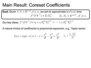
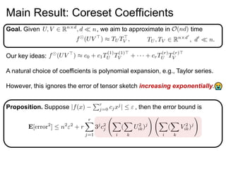
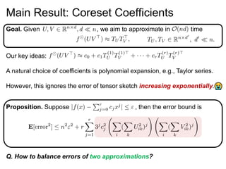
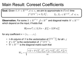
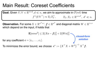
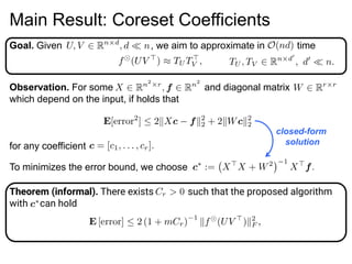
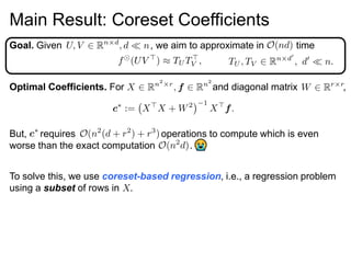
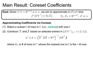
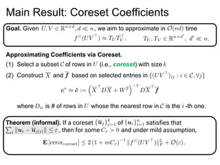
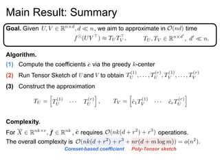
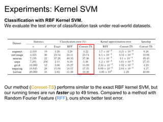
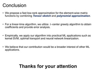
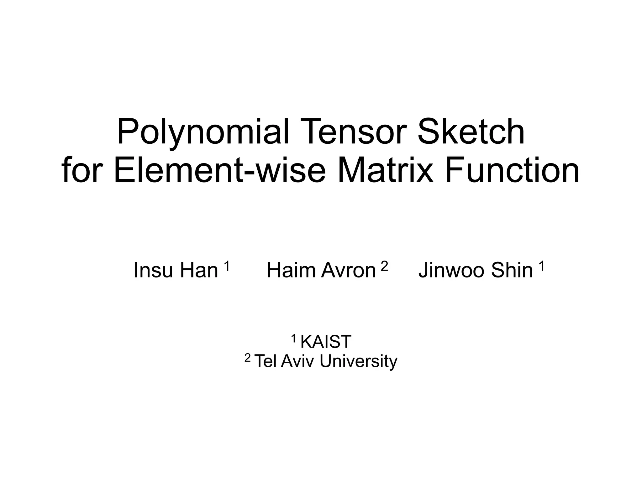
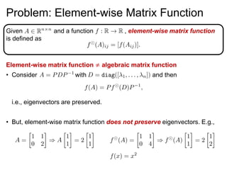
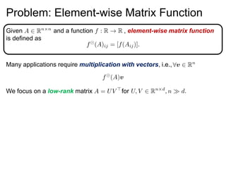
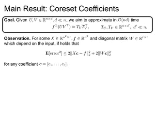
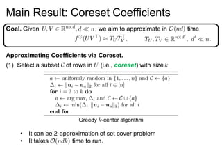
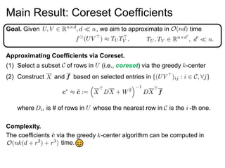
1) The document proposes a polynomial tensor sketch method to approximate element-wise matrix functions in linear time. It combines tensor sketching, which can approximate matrix monomials fast, with polynomial approximation of the target function. 2) Coreset-based regression is used to efficiently compute optimal polynomial coefficients by selecting a small subset of rows. 3) Experiments show the method outperforms alternatives like random Fourier features for applications like kernel approximation, kernel SVM, and Sinkhorn algorithm, providing speedups of up to 49x.

1. Polynomial Tensor Sketch
for Element-wise Matrix Function
Insu Han 1 Haim Avron 2 Jinwoo Shin 1
1 KAIST
2 Tel Aviv University

2. Problem: Element-wise Matrix Function
Example:
Given and a function , element-wise matrix function
is defined as

3. Problem: Element-wise Matrix Function
Applications in machine learning
• Non-linear activation functions in deep learning:
• Kernel methods (e.g., Gaussian process, Determinantal Point Process):
(MLP)
(Transformer)
Given and a function , element-wise matrix function
is defined as

4. Problem: Element-wise Matrix Function
Element-wise matrix function ≠ algebraic matrix function
• Consider with and then
i.e., eigenvectors are preserved.
• But, element-wise matrix function does not preserve eigenvectors. E.g.,
Given and a function , element-wise matrix function
is defined as

5. Many applications require multiplication with vectors, i.e.,
We focus on a low-rank matrix for
Problem: Element-wise Matrix Function
Given and a function , element-wise matrix function
is defined as

6. Many applications require multiplication with vectors, i.e.,
We focus on a low-rank matrix for
Problem: Element-wise Matrix Function
Issue. It requires complexity to compute, too expensive for large .
Goal. Design a fast algorithm of time-complexity
for low-rank approximation of ,
i.e., without computing all entries of .
Given and a function , element-wise matrix function
is defined as

7. Main Result: Polynomial Tensor Sketch
Our key ideas:
1. Tensor sketch [PP13] can approximate element-wise matrix monomial
function in time, i.e.,
Goal. Given , we aim to approximate in time

8. Main Result: Polynomial Tensor Sketch
Our key ideas:
1. Tensor sketch [PP13] can approximate element-wise matrix monomial
function in time, i.e.,
2. Polynomial approximation on
Goal. Given , we aim to approximate in time

9. Main Result: Polynomial Tensor Sketch
Our key ideas:
1. Tensor sketch [PP13] can approximate element-wise matrix monomial
function in time.
2. Polynomial approximation on
Applying Tensor sketch with , the low-rank approximation on
can be done in time.
target dimension for Tensor sketch
polynomial degree
Goal. Given , we aim to approximate in time

10. Main Result: Polynomial Tensor Sketch
Our key ideas:
1. Tensor sketch [PP13] can approximate element-wise matrix monomial
function in time.
2. Polynomial approximation on
Applying Tensor sketch with , the low-rank approximation on
can be done in time.
Q. How can find good coefficients?
target dimension for Tensor sketch
polynomial degree
Goal. Given , we aim to approximate in time

11. Main Result: Coreset Coefficients
Our key ideas:
A natural choice of coefficients is polynomial expansion, e.g., Taylor series.
Goal. Given , we aim to approximate in time

12. Main Result: Coreset Coefficients
Our key ideas:
A natural choice of coefficients is polynomial expansion, e.g., Taylor series.
However, this ignores the error of tensor sketch increasing exponentially.
Proposition. Suppose , then the error bound is
Goal. Given , we aim to approximate in time

13. Main Result: Coreset Coefficients
Our key ideas:
A natural choice of coefficients is polynomial expansion, e.g., Taylor series.
However, this ignores the error of tensor sketch increasing exponentially.
Q. How to balance errors of two approximations?
Goal. Given , we aim to approximate in time
Proposition. Suppose , then the error bound is

14. Main Result: Coreset Coefficients
Observation. For some and diagonal matrix
which depend on the input, if holds that
for any coefficient
Goal. Given , we aim to approximate in time

15. Main Result: Coreset Coefficients
• -th column of is the vectorization of for all
• is the vectorization of
• is the diagonal matrix such that
Goal. Given , we aim to approximate in time
Observation. For some and diagonal matrix
which depend on the input, if holds that
for any coefficient

16. Main Result: Coreset Coefficients
To minimizes the error bound, we choose
closed-form
solution
Goal. Given , we aim to approximate in time
Observation. For some and diagonal matrix
which depend on the input, if holds that
for any coefficient

17. Main Result: Coreset Coefficients
Observation. For some and diagonal matrix
which depend on the input, if holds that
for any coefficient
To minimizes the error bound, we choose
Goal. Given , we aim to approximate in time
closed-form
solution
Theorem (informal). There exists such that the proposed algorithm
with can hold

18. Main Result: Coreset Coefficients
Optimal Coefficients. For and diagonal matrix ,
But, requires operations to compute which is even
worse than the exact computation .
Goal. Given , we aim to approximate in time

19. Main Result: Coreset Coefficients
To solve this, we use coreset-based regression, i.e., a regression problem
using a subset of rows in .
Goal. Given , we aim to approximate in time
Optimal Coefficients. For and diagonal matrix ,
But, requires operations to compute which is even
worse than the exact computation .

20. Main Result: Coreset Coefficients
Approximating Coefficients via Coreset.
(1) Select a subset of rows in (i.e., coreset) with size
(2) Construct and based on selected entries in
where is # of rows in whose the nearest row in is the -th one.
Goal. Given , we aim to approximate in time

21. Main Result: Coreset Coefficients
Goal. Given , we aim to approximate in time
Approximating Coefficients via Coreset.
(1) Select a subset of rows in (i.e., coreset) with size
(2) Construct and based on selected entries in
where is # of rows in whose the nearest row in is the -th one.
Theorem (informal). If a coreset of satisfies that
, then for some and under mild assumption,

22. Main Result: Coreset Coefficients
Approximating Coefficients via Coreset.
(1) Select a subset of rows in (i.e., coreset) with size
• It can be 2-approximation of set cover problem
• It takes time to run.
Goal. Given , we aim to approximate in time
Greedy -center algorithm

23. Main Result: Coreset Coefficients
Approximating Coefficients via Coreset.
(1) Select a subset of rows in (i.e., coreset) via the greedy -center
(2) Construct and based on selected entries in
where is # of rows in whose the nearest row in is the -th one.
Goal. Given , we aim to approximate in time
Complexity.
The coefficients via the greedy -center algorithm can be computed in
time.

24. Main Result: Summary
Algorithm.
(1) Compute the coefficients via the greedy -center
(2) Run Tensor Sketch of and to obtain
(3) Construct the approximation
For , requires operations.
The overall complexity is
Coreset-based coefficient Poly-Tensor sketch
Complexity.
Goal. Given , we aim to approximate in time

25. Experiments: Kernel Approximation
RBF Kernel Approximation.
Our method (Coreset-TS) outperforms other competitors; random Fourier
feature (RFF), and algorithm with coefficient from Taylor (Taylor-TS) and
Chebyshev series (Chebyshev-TS).

26. Experiments: Kernel SVM
Classification with RBF Kernel SVM.
We evaluate the test error of classification task under real-world datasets.
Our method (Coreset-TS) performs similar to the exact RBF kernel SVM, but
our running times are run faster up to 49 times. Compared to a method with
Random Fourier Feature (RFF), ours show better test error.

27. Experiments: Sinkhorn Algorithm
Sinkhorn Algorithm for Computing Optimal Transport Distance.
Given vectors and a low-rank matrix , Sinkhorn requires to compute
We evaluate speed up and approximation ratio of Random Fourier Feature
(RFF), Nystrom method and our algorithm (Coreset-TS) to image color
transformation. Ours show the smallest variance on approximation ratio.

28. Experiments: Neural Network Linearization
Linearization of Neural Network.
Given a 2-layer fully-connected network, a low-rank approximation on non-
linear operation can be linearized the network:
• (+) The inference time can be reduced once parameters are pre-computed
• (−) The inputs should be computed with non-linear transform, i.e.,
Results on final 2 FC layers of AlexNet trained by CIFAR10 dataset

29. Conclusion
• We propose a fast low-rank approximation for the element-wise matrix
functions by combining Tensor sketch and polynomial approximation.
• For a linear-time algorithm, we utilize -center greedy algorithm to obtain
coefficients and provide error analysis.
• Empirically, we apply our algorithm into practical ML applications such as
kernel SVM, optimal transport and neural network linearization.
• We believe that our contribution would be a broader interest of other ML
applications.
Thanks for your attention