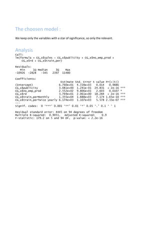
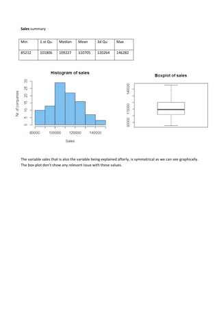
The document describes a multiple regression model that was constructed to best explain sales using data from a file. The model's formal equation shows sales as a function of several independent variables including publicity, number of employees in administration and production, expenditure on research and development, income, seniority, number of products, training start time, and training period. The results of the analysis show that publicity, number of employees in production, expenditure on R&D, and training period are significant predictors of sales in the model.

1. Student: Carmine Gelormini
Final project for Econometrics.
A model which best explains sales it’s constructed using the data from the file “Data set n17.csv”.
Description of the data:
The sample have 100 observation per each of the 10 variables. Each observation refers to a specific
company (e.g. “company1”,” company2”,…, “company100”)
Descriptive indicators: min, max, mean, median and quartiles;
Publicity summaries
Figura 1.1 summary of the variables

2. The mean for the variable “publicity”, showed in the summary table, tells us that
the most of the companies spend about 18520 units ( of the reference currency) on
advertising. The minimum expenditure it’s 14336 units while the maximum it’s
29765. The median it’s close to the mean value, being equal to 19213, can led us
think of a normal distribuited data, but instead the shape as we can see in the first
graph is more positively asimetrical, with most part of the values being in the first
half of the distribution. Also the stat. 1st Qu. ( “first quartile”) tells us that the a first
25% of the companies spend between 14336 and 16215 units, while the 3rd Qu.
means that the considering the total 75% of the values the max. it’s 21307. Those
are best visualized whithin the box-plot. We can see that the top whirsk is loger than
the first, while the box at the center it’s located toward the bottom of the space.
This box indicate the most of the value of the distribution.
No_emp_admin summaries
Min. 1.st
Qu.
Media
n
Mean 3d Qu Max
14336 16215 18520 19213 21307 29765

3. T
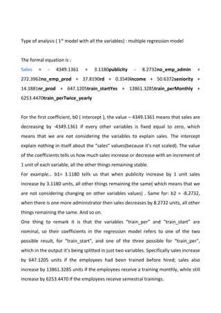
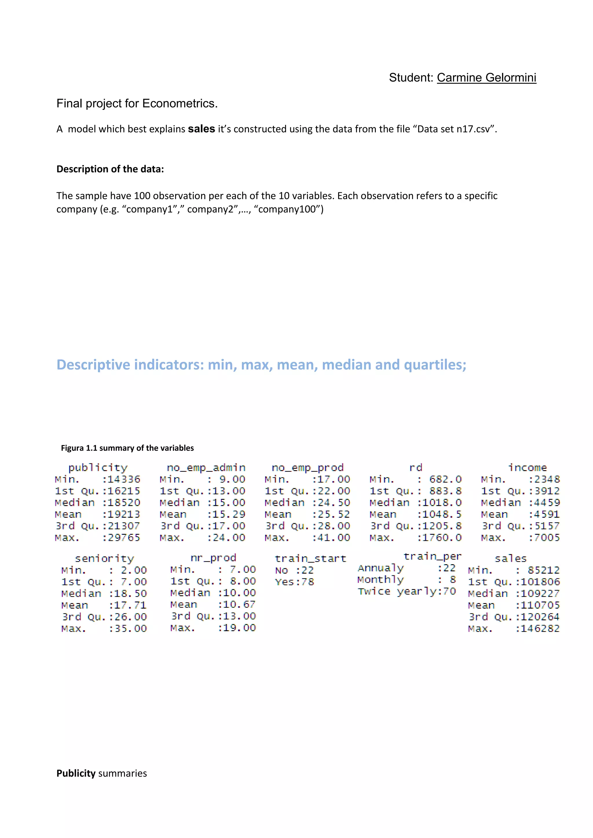
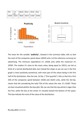
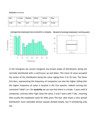
The variable “no_emp_admin” the mean is located around the 15.29 value, which
correspond to an average of 15 administrator working in the company. As the
previous min. and max. value tells us only the extreme points. The median it’s close
to the mean value, being equal to 15. Looking at the histogram and also with the
help of these basical statistics we note, by the way, that the shape of the
distribution is normal but we can’t say this variable is normally distributed because
the mode, which is 14 here [<- table(CG_x$no_emp_admin)], don’t correspond to
the mean and the median. The interpretation of the stat. 1st
Qu. and the 3rd
Qu. it’s
similar to the previous variable, but being more centered to the middle of the space.
We still note an outlier ( a very high or very low value) after the top whisker.
No_emp_prod summaries
Min. 1.st
Qu.
Media
n
Mean 3d Qu Max
9.00 13.00 15.00 15.29 17.00 24.00

4. Methodologically this variable have the same attributes as the previous one, but
measuring the emplooyes involved in the production, the general values will be
higher. The graphical shape looks also like a normal curve, slightly positively
asymmetrical with a right tail. The range of values goes from 17 to 41, but the 1st
and 3rd
quartiles tells us that the most of the companies have between 22 and 28
workers involved in the production, as the box-plot will better visualize.
Min. 1.st
Qu.
Media
n
Mean 3d Qu Max
17.00 22.00 24.50 25.52 28.00 41.00

5. Expenditure on research and development summaries
Slightly different are the values for the variable rd, being more spread whithin the
total. The most of the companies spend around 1048.5 units on research and
development. Overally all the companies are spending less on research and
development that what they spend for publicity. The shape of distribution looks like
symmetrical, with more than one level of expenditure in which companies are
aligned.
Again we have a majority of the values located around the mean, as we see in the
box-plot, two differently sloped tails and an outlier over the 75% of the distribution.
Min. 1.st Qu. Median Mean 3d Qu Max
682.0 883.8 1018 1048.5 12.05.8 1760

6. The variable income it’s very near to be perfectly simmetrical distribuited, being
mean, median and mode almost on the same value. The values represents which
level of income have the clients of each company. Being so predictable, it has to be
noted that the values after the median are more spread. We don’t have any outlier
in the box plot here.
Min. 1.st Qu. Median Mean 3d Qu Max
2348 3912 4459 4591 5157 7005

7. Seniority summaries
In the histogram we cannot recognize any known shape of distribution, being not
normally distributed with a continuous up and down. The mean of value occupied
the center of the distribution being the value raging from 2 to 35 max. The three
first bars, representing the frequency of companies are also the higher telling that
the higher frequency of value is located in the first quarter. Indeed running the
command “table” on r for seniority we can see that there is a mode, 7 years with 8
companies, and two other high value the same, 3 and 7 years with 7 obs. ,meaning
that usually the employees work for little years The box- plot shows a very spread
distribution more extended almost equally divided totally, but if considering only
the .
Min. 1.st Qu. Median Mean 3d Qu Max
2.00 7.00 18.5 17.71. 26.00 35.00

8. Nr_products summary
Fairly easy to interpret is the statistic on the
variable nr. of products, being purely numerical the same, but also showing that the
majority of the companies don’t sell a large set of products. The distribution is
positively asimetrical with a right tail fairly descending after the mode of 8 products
by more than 15 companies. The arithmetic mean by the way it’s 10.67 due to a
group of observation that range from 9 to 12 units and have a similar frequency.
Min. 1.st Qu. Median Mean 3d Qu Max
7.00 8.00 10.00 10.67 13.00 19.00

9. For the two nominal variables we don’t have a summary, being this variable directly
looked on the bar-plot which serve as a frequency table also.

10. Sales summary
The variable sales that is also the variable being explained afterly, is symmetrical as we can see graphically.
The box-plot don’t show any relevant issue with these values.
Min. 1.st Qu. Median Mean 3d Qu Max
85212 101806 109227 110705 120264 146282

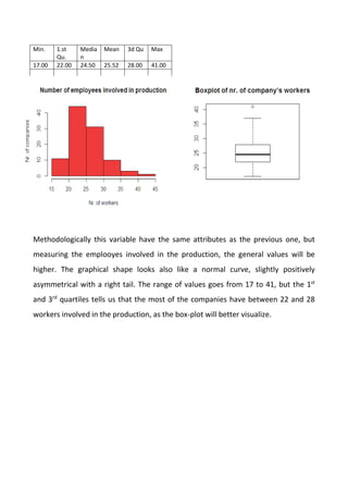
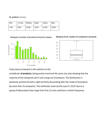
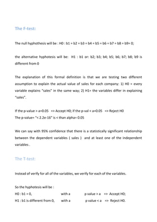
11. We will start now to look at the coefficients of correlation to see. These tells us
about the association between two variables. Remembering that association doesn’t
mean causation, one should look for the high scores on these coefficients for the
starting point for find pattern of relationships. This coefficient goes by -1 to +1. A
score of 0 or around 0 indicate no correlation, while from the 0 towards the two
extreme, a firstly weak and then high correlation.
Placed side by side are also the scatter-plot showing the distribution of the
points/unit on the two dimentional space of the correlated variables.
> cor(CG_x$sales,CG_x$publ
icity)
[1] 0.7163831
There is a strong positive
correlation between the tw
o variables, that means th
at when publicity increase
also sales are lifting up.
> cor(CG_x$sales,CG_x$no_emp_
admin)
[1] 0.1124151
There is no correlation. This means
that when sales increase the other
variables don’t have a unique way of
changing.

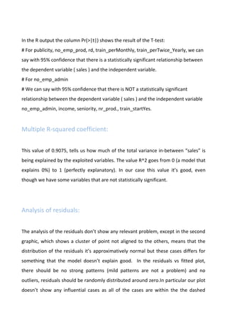
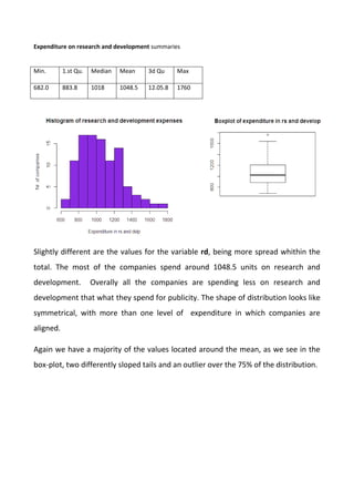
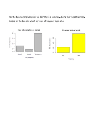
12. cor(CG_x$sales,CG_x$no_emp_
prod)
[1] -0.07883389
There is no correlation. Even looking
at the plot, every point is spread
almost randomly and there are not
graphically recognising patterns.
> cor(CG_x$sales,CG_x$rd)
[1] 0.5212227
This value indicated a weak positive
correlation, meaning that when rd
increases sales also increase with a
slightly slope.
cor(CG_x$sales,CG_x$seniority
)
[1] -0.06973496
The variables are not correlated.

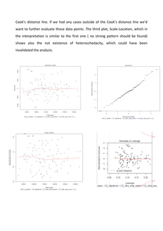
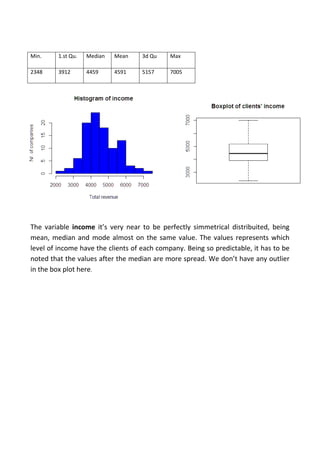
13. Interpretation of the results:
Call:
lm(formula = CG_x$sales ~ CG_x$publicity + CG_x$no_emp_admin +
CG_x$no_emp_prod + CG_x$rd + CG_x$income + CG_x$seniority +
CG_x$nr_prod + CG_x$train_start + CG_x$train_per)
Residuals:
Min 1Q Median 3Q Max
-10585.3 -2816.7 -25.5 2267.0 11254.3
Coefficients:
Estimate Std. Error t value Pr(>|t|)
(Intercept) -4349.1361 6630.2751 -0.656 0.51355
CG_x$publicity 3.1180 0.1284 24.291 < 2e-16 ***
CG_x$no_emp_admin -8.2732 143.4006 -0.058 0.95412
CG_x$no_emp_prod 272.3962 101.3058 2.689 0.00856 **
CG_x$rd 37.8190 2.2820 16.572 < 2e-16 ***
CG_x$income 0.3549 0.5139 0.691 0.49160
CG_x$seniority 50.6372 47.5523 1.065 0.28981
CG_x$nr_prod 14.1881 170.2947 0.083 0.93379
CG_x$train_startYes 647.1205 1108.5769 0.584 0.56087
CG_x$train_perMonthly 13861.3285 1941.1590 7.141 2.42e-10 ***
CG_x$train_perTwice yearly 6253.4470 1135.3762 5.508 3.48e-07 ***
---
Signif. codes: 0 ‘***’ 0.001 ‘**’ 0.01 ‘*’ 0.05 ‘.’ 0.1 ‘ ’ 1
Residual standard error: 4509 on 89 degrees of freedom
Multiple R-squared: 0.9075, Adjusted R-squared: 0.8971
F-statistic: 87.33 on 10 and 89 DF, p-value: < 2.2e-16
2.1 results of the analysis (from R output)
> cor(CG_x$sales,CG_x$nr_pr
od)
[1] -0.2052322
Not correlated.

14. Type of analysis ( 1st
model with all the variables) : multiple regression model
The formal equation is :
Sales = - 4349.1361 + 3.1180publicity - 8.2732no_emp_admin +
272.3962no_emp_prod + 37.8190rd + 0.3549income + 50.6372seniority +
14.1881nr_prod + 647.1205train_startYes + 13861.3285train_perMonthly +
6253.4470train_perTwice_yearly
For the first coefficient, b0 ( intercept ), the value – 4349.1361 means that sales are
decreasing by -4349.1361 if every other variables is fixed equal to zero, which
means that we are not considering the variables to explain sales. The intercept
explain nothing in itself about the “sales” values(because it’s not scaled). The value
of the coefficients tells us how much sales increase or decrease with an increment of
1 unit of each variable, all the other things remaining stable.
For example… b1= 3.1180 tells us that when publicity increase by 1 unit sales
increase by 3.1180 units, all other things remaining the same( which means that we
are not considering changing on other variables values) . Same for: b2 = -8.2732,
when there is one more administrator then sales decreases by 8.2732 units, all other
things remaining the same. And so on.
One thing to remark it is that the variables “train_per” and “train_start” are
nominal, so their coefficients in the regression model refers to one of the two
possible result, for “train_start”, and one of the three possible for “train_per”,
which in the output it’s being splitted in just two variables. Specifically sales increase
by 647.1205 units if the employees had been trained before hired; sales also
increase by 13861.3285 units if the employees receive a training monthly, while still
increase by 6253.4470 if the employees receive semestral trainings.

15. The F-test:
The null hyphothesis will be : H0 : b1 = b2 = b3 = b4 = b5 = b6 = b7 = b8 = b9= 0;
the alternative hyphotesis will be: H1 : b1 or: b2; b3; b4; b5; b6; b7; b8; b9 is
different from 0
The explanation of this formal definition is that we are testing two different
assumption to explain the actual value of sales for each company: 1) H0 = every
variable explains “sales” in the same way; 2) H1= the variables differ in explaining
“sales”.
If the p-value > a=0.05 => Accept H0; if the p-val < a=0.05 => Reject H0
The p-value= “< 2.2e-16” is < than alpha= 0.05
We can say with 95% confidence that there is a statistically significant relationship
between the dependent variables ( sales ) and at least one of the independent
variables .
The T-test:
Instead of verify for all of the variables, we verify for each of the variables.
So the hyphotesis will be :
H0 : b1 = 0, with a p value > a => Accept H0;
H1 : b1 is different from 0, with a p value < a => Reject H0.

16. In the R output the column Pr(>|t|) shows the result of the T-test:
# For publicity, no_emp_prod, rd, train_perMonthly, train_perTwice_Yearly, we can
say with 95% confidence that there is a statistically significant relationship between
the dependent variable ( sales ) and the independent variable.
# For no_emp_admin
# We can say with 95% confidence that there is NOT a statistically significant
relationship between the dependent variable ( sales ) and the independent variable
no_emp_admin, income, seniority, nr_prod., train_startYes.
Multiple R-squared coefficient:
This value of 0.9075, tells us how much of the total variance in-between “sales” is
being explained by the exploited variables. The value R^2 goes from 0 (a model that
explains 0%) to 1 (perfectly explanatory). In our case this value it’s good, even
though we have some variables that are not statistically significant.
Analysis of residuals:
The analysis of the residuals don’t show any relevant problem, except in the second
graphic, which shows a cluster of point not aligned to the others, means that the
distribution of the residuals it’s approximatively normal but these cases differs for
something that the model doesn’t explain good. In the residuals vs fitted plot,
there should be no strong patterns (mild patterns are not a problem) and no
outliers, residuals should be randomly distributed around zero.In particular our plot
doesn’t show any influential cases as all of the cases are within the the dashed

17. Cook’s distance line. If we had any cases outside of the Cook’s distance line we’d
want to further evaluate those data points. The third plot, Scale-Location, which in
the interpretation is similar to the first one ( no strong pattern should be found)
shows also the not existence of heteroschedacity, which could have been
invalidated the analysis.

18. The choosen model :
We keep only the variables with a star of significance, so only the relevant.
Analysis
Call:
lm(formula = CG_x$sales ~ CG_x$publicity + CG_x$no_emp_prod +
CG_x$rd + CG_x$train_per)
Residuals:
Min 1Q Median 3Q Max
-10926 -2828 -345 2397 11480
Coefficients:
Estimate Std. Error t value Pr(>|t|)
(Intercept) 6.760e+01 4.728e+03 0.014 0.9886
CG_x$publicity 3.081e+00 1.241e-01 24.831 < 2e-16 ***
CG_x$no_emp_prod 2.552e+02 9.806e+01 2.603 0.0107 *
CG_x$rd 3.769e+01 2.061e+00 18.284 < 2e-16 ***
CG_x$train_perMonthly 1.355e+04 1.888e+03 7.174 1.65e-10 ***
CG_x$train_perTwice yearly 6.174e+03 1.107e+03 5.578 2.33e-07 ***
---
Signif. codes: 0 ‘***’ 0.001 ‘**’ 0.01 ‘*’ 0.05 ‘.’ 0.1 ‘ ’ 1
Residual standard error: 4445 on 94 degrees of freedom
Multiple R-squared: 0.9051, Adjusted R-squared: 0.9
F-statistic: 179.2 on 5 and 94 DF, p-value: < 2.2e-16

19. Interpretation
Now for the first coefficient, b0 ( intercept ), the value 67.60 means that sales are increasing by
67.60 if every other variables is fixed equal to zero. The same criteria of interpretation applies to
the other listed coefficients. As we can realize we have a more likely explanation of the “sales”
variables, with all of the independent variables being statistically significant in the F-test and the T-
test, wich mean that we have a statistically significant evidence for a relationship between the
dependent and the independent variables.
Almost nothing changes for the R^2 coefficient, being equal to 0.90. The same interpretation as the
previous model follows for the analysis of the residuals.