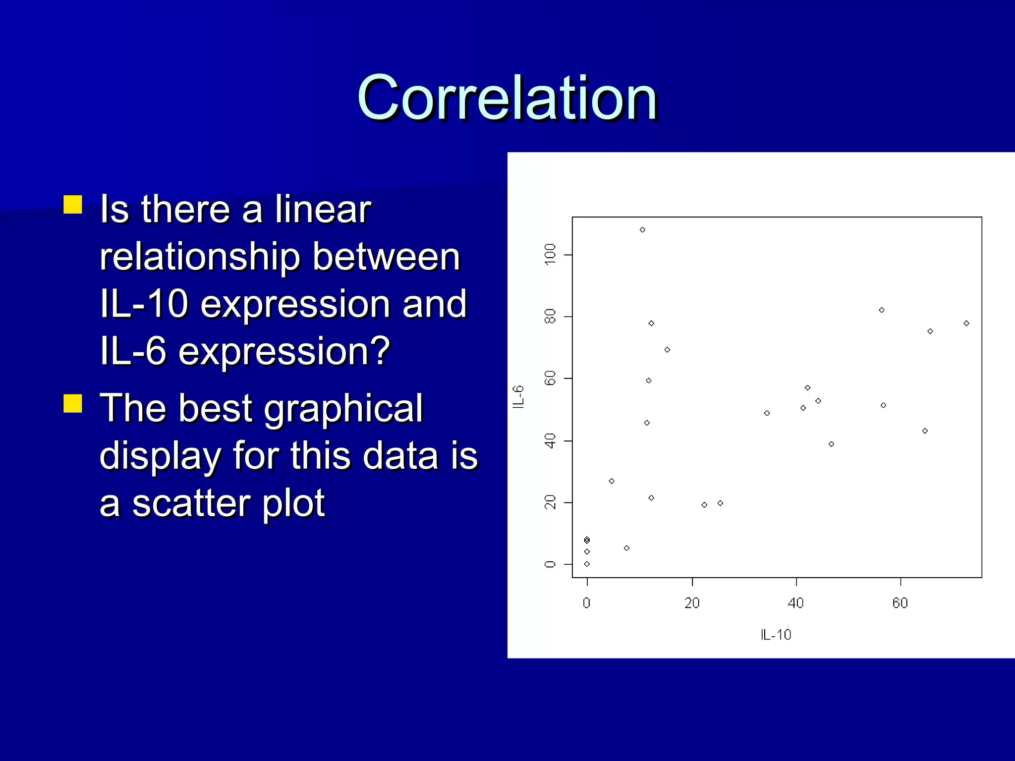
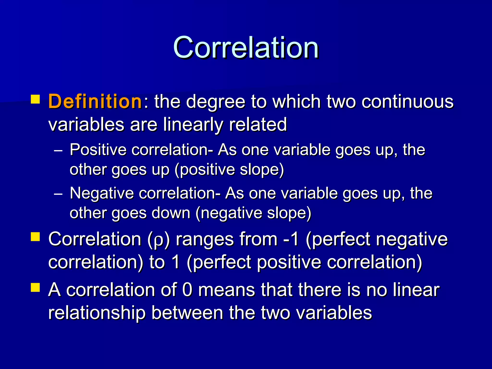
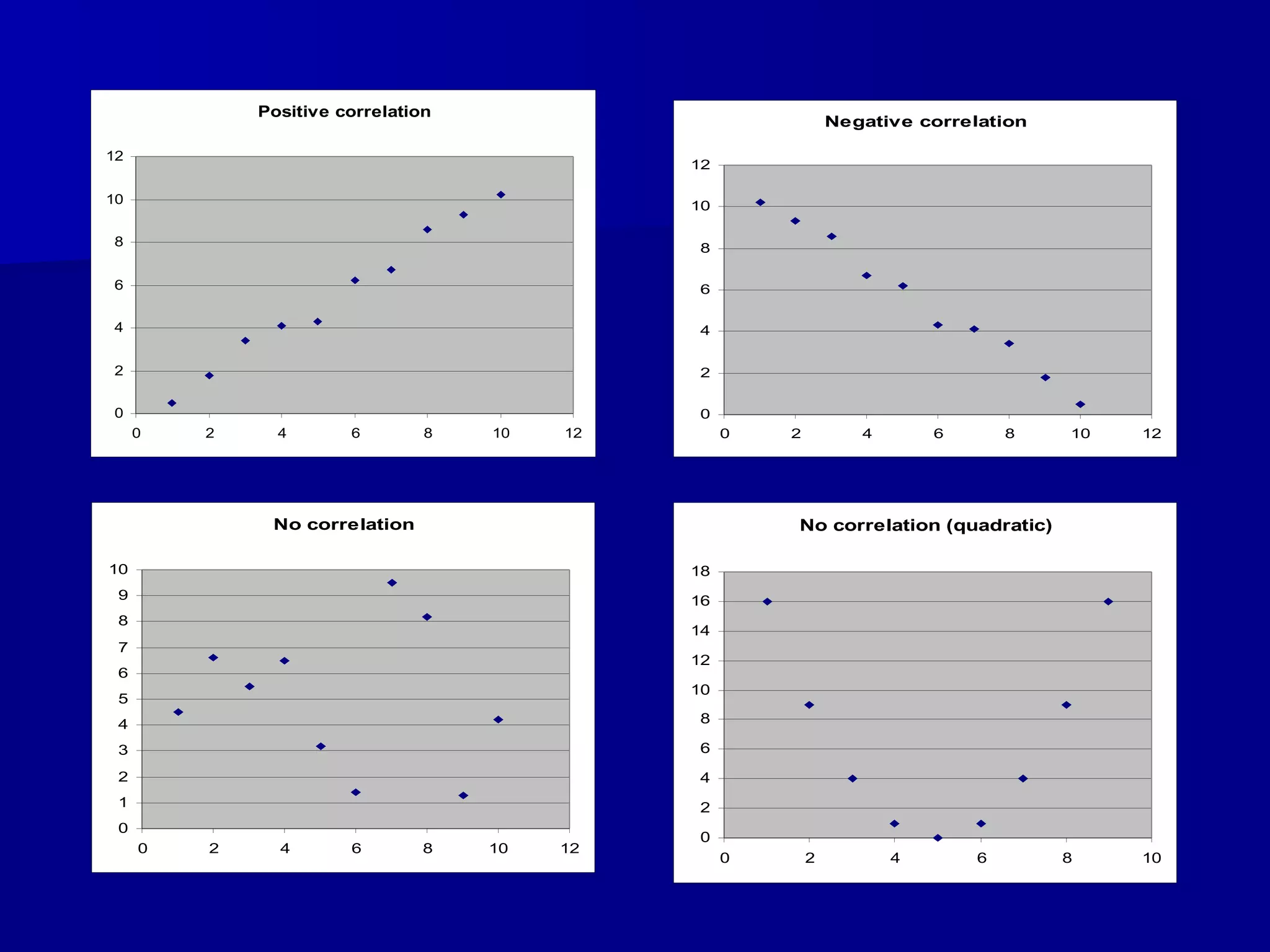
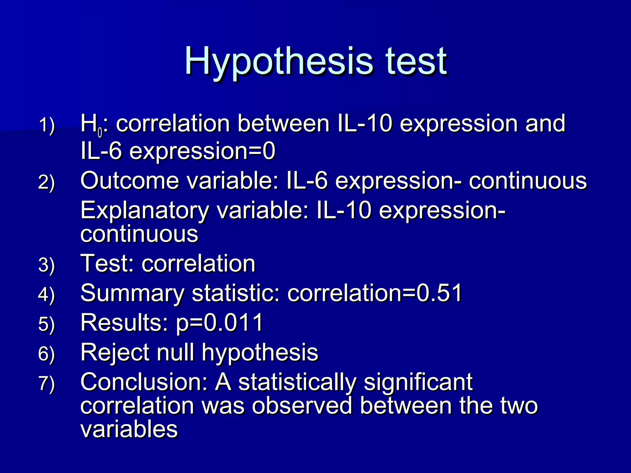
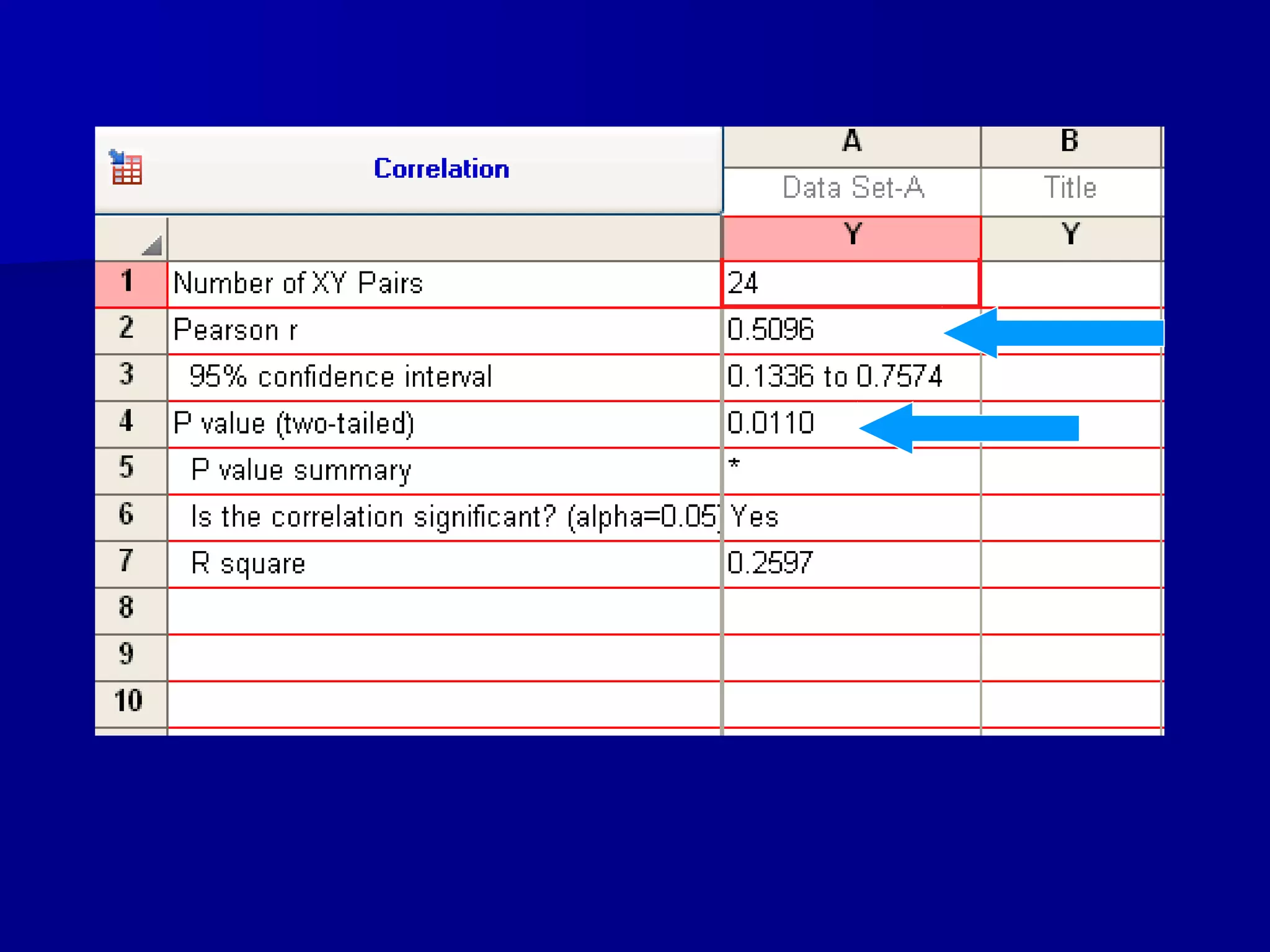
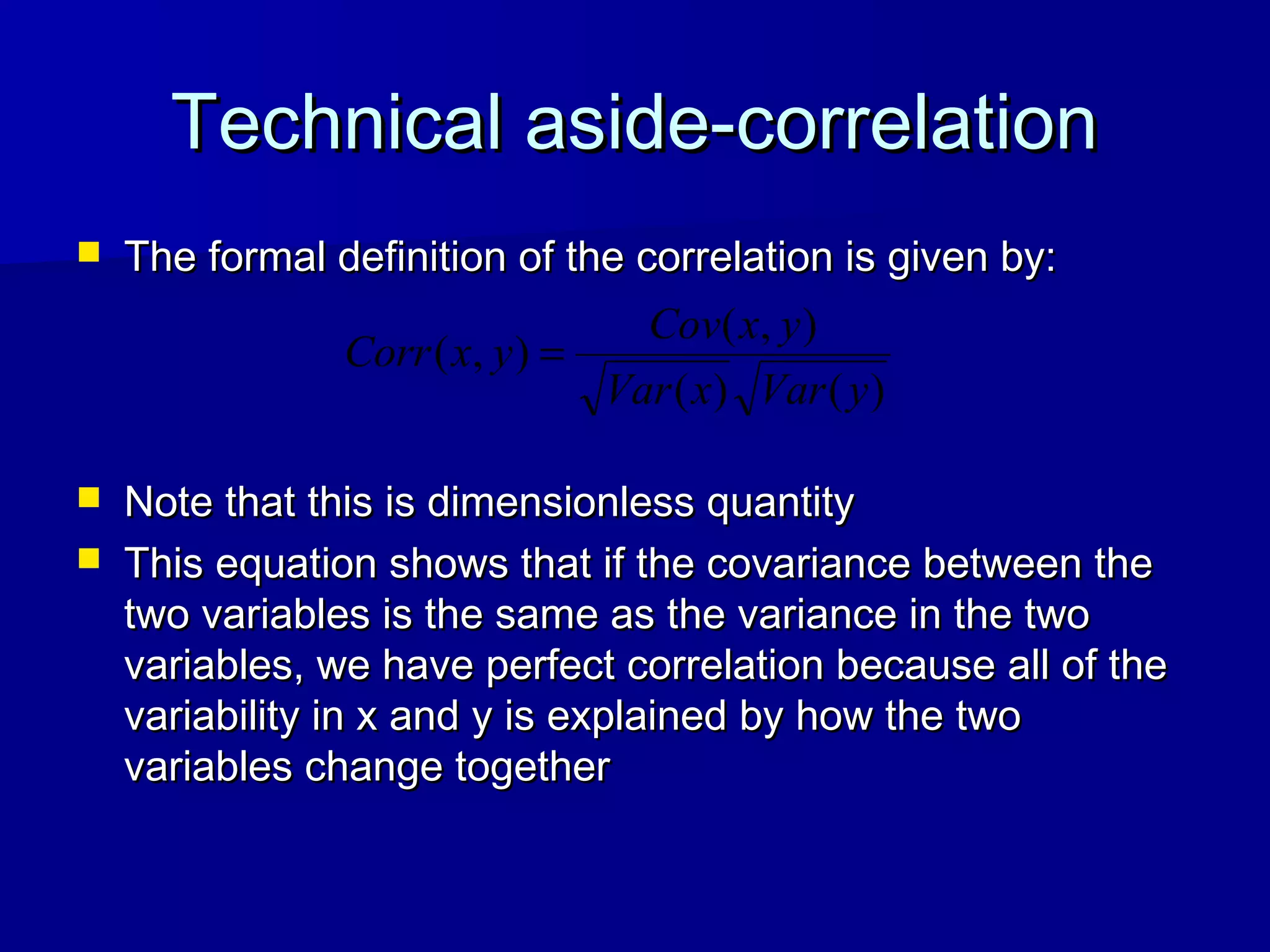
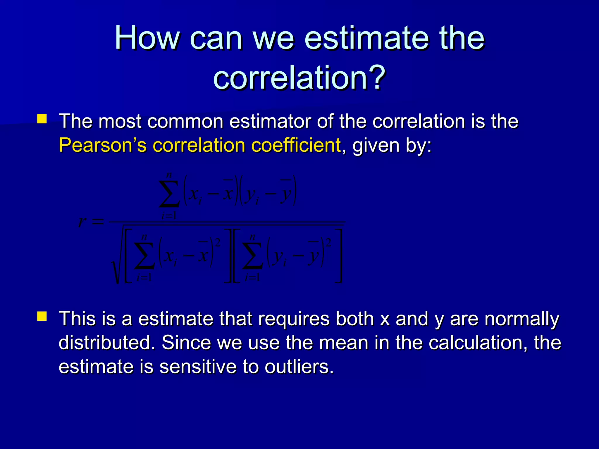
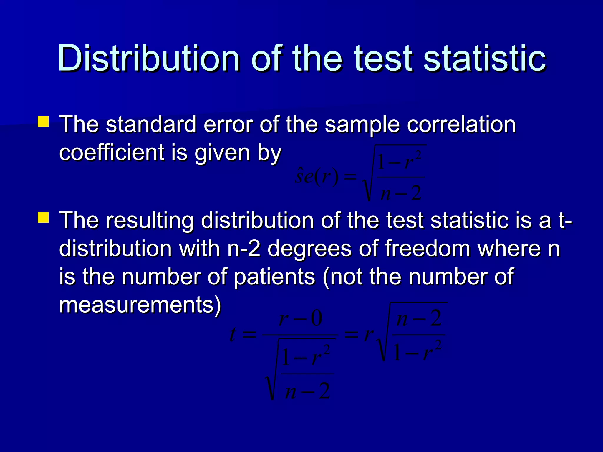
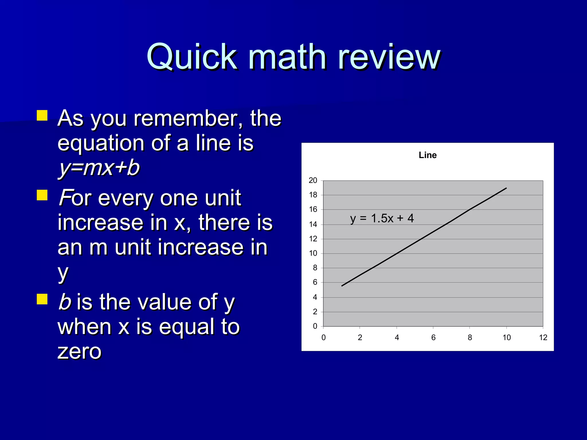
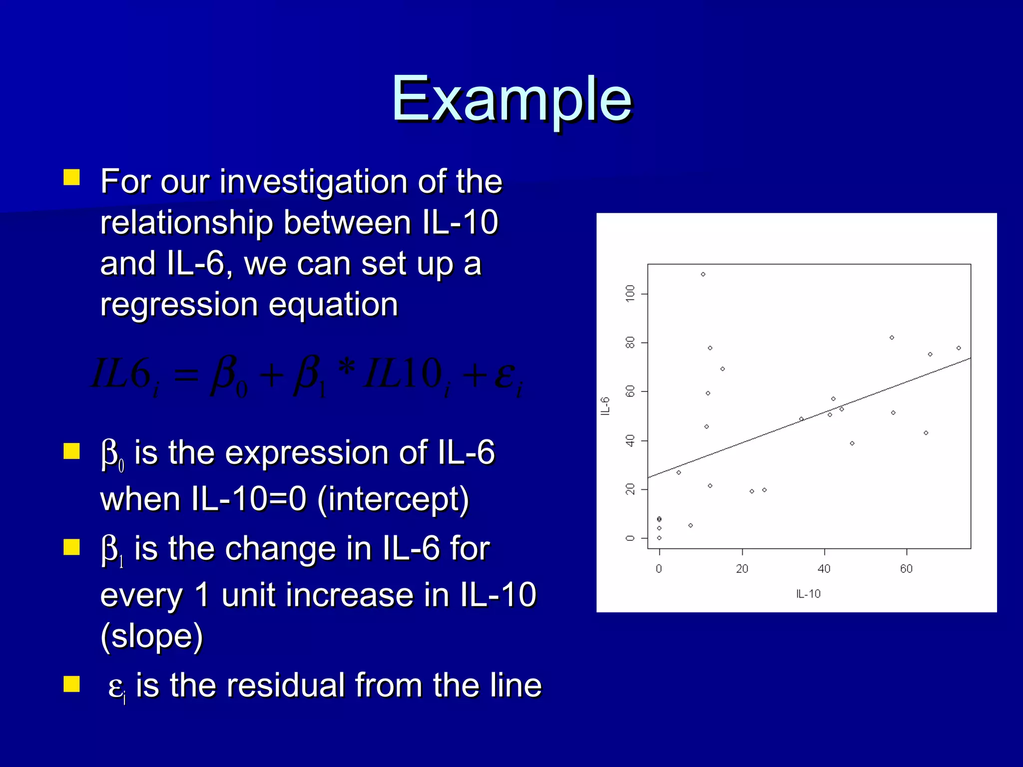
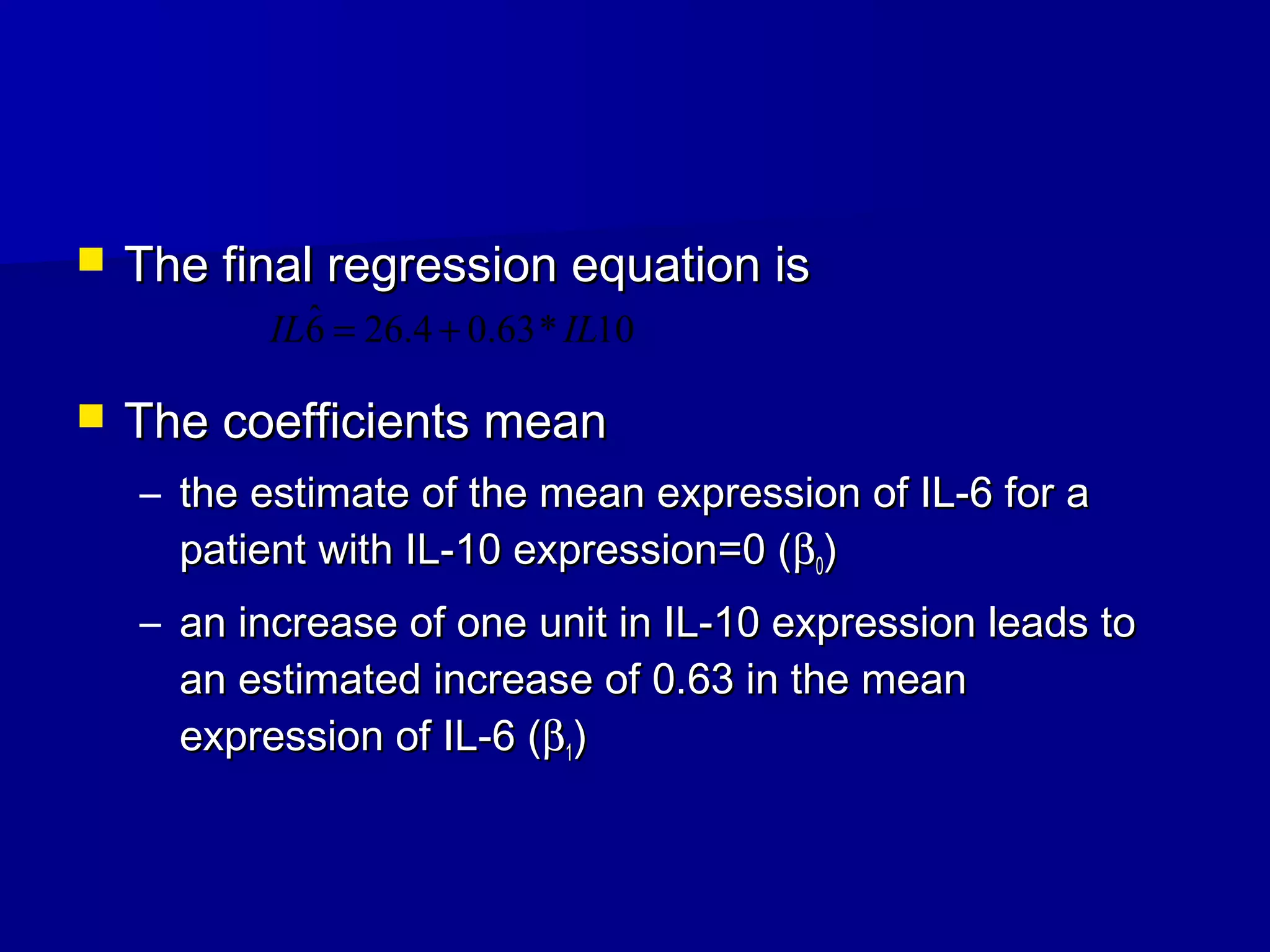
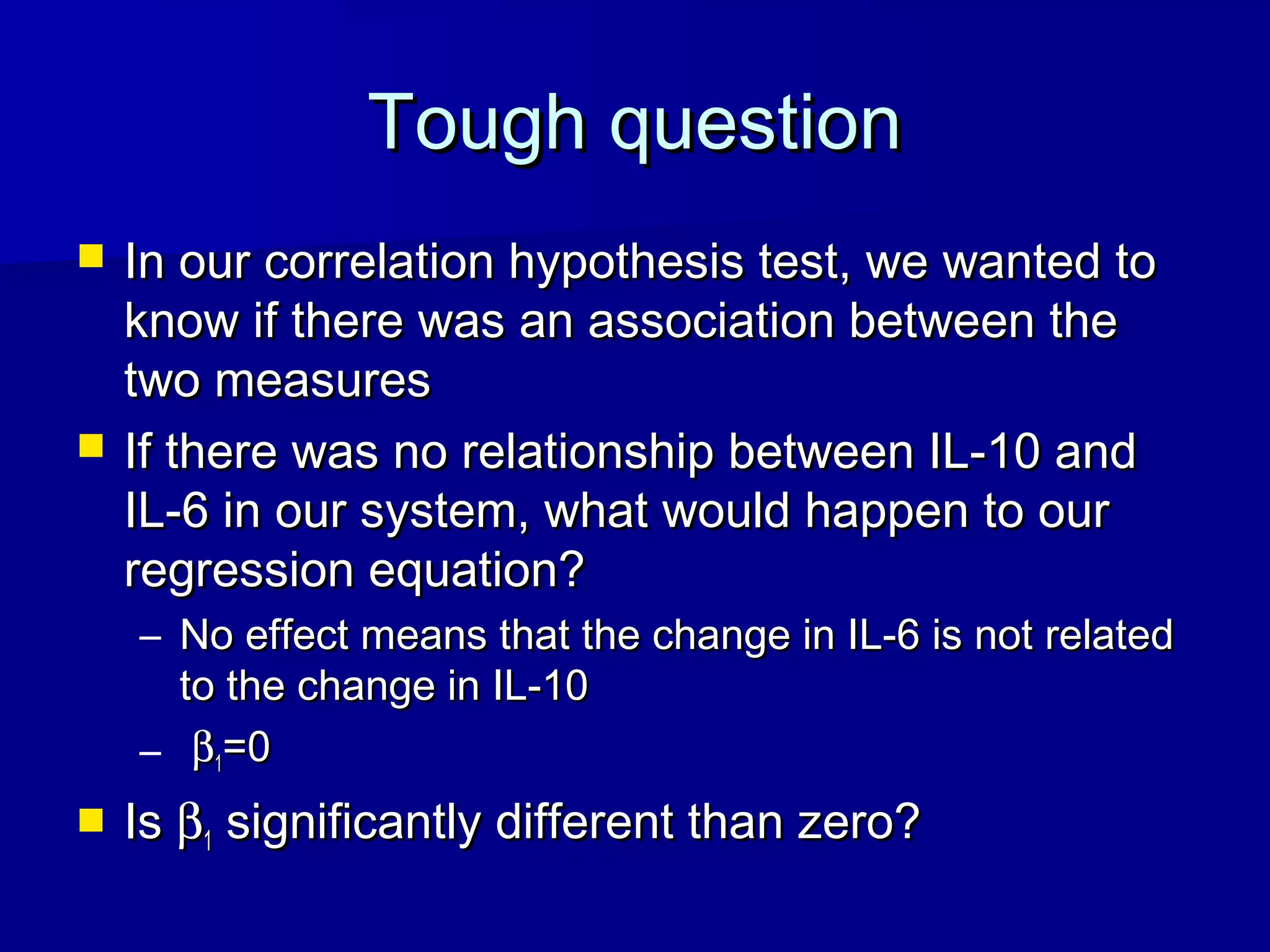
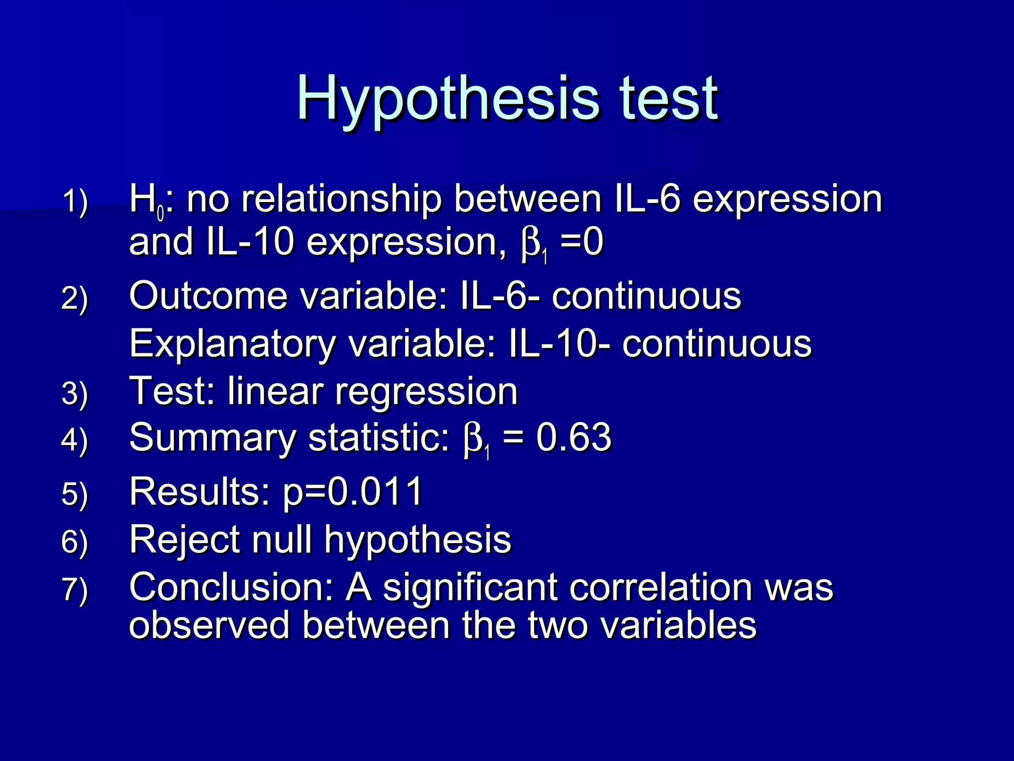
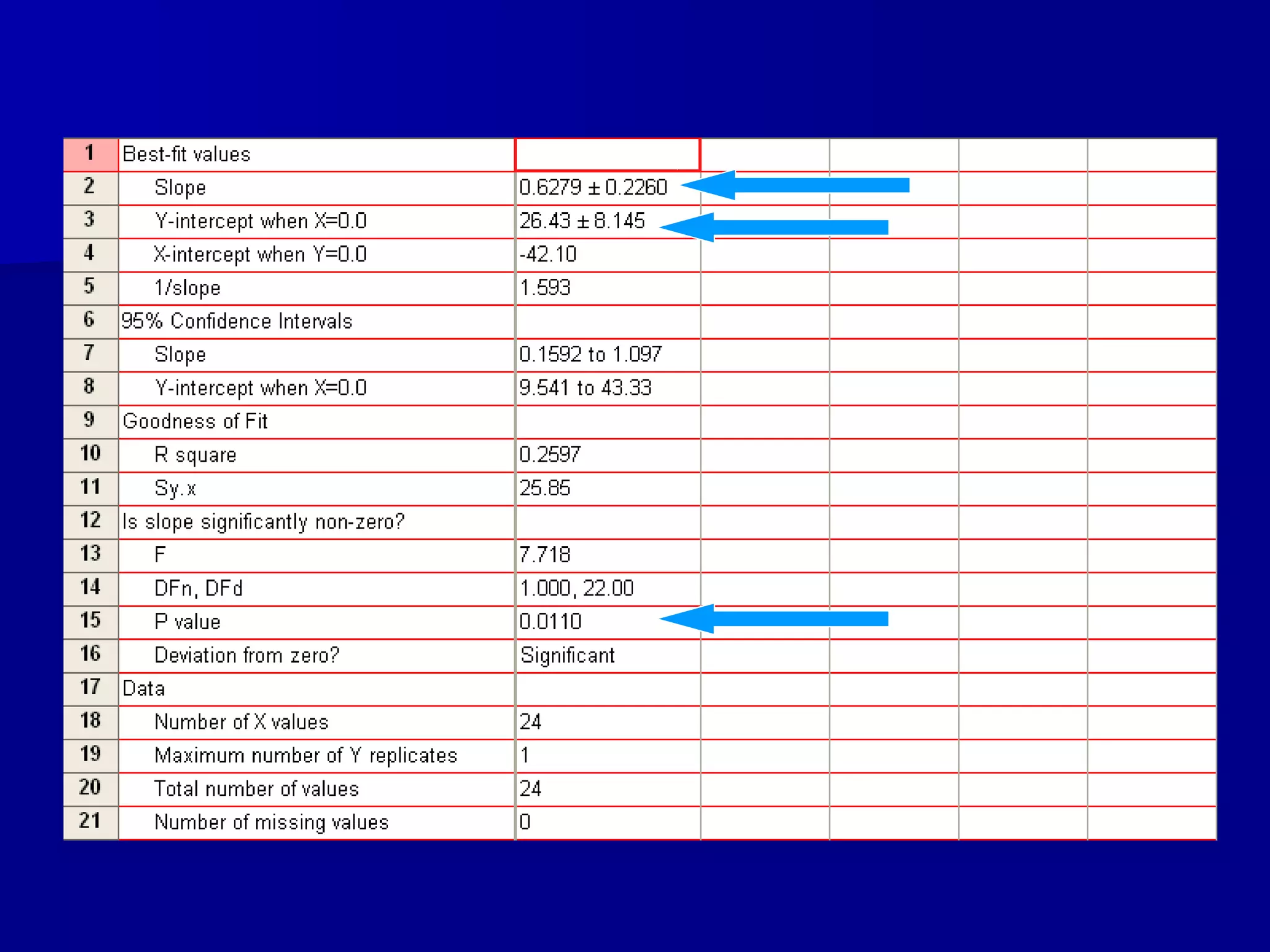
1. ReviewReview
Types of dataTypes of data
p-valuep-value
Steps for hypothesis testSteps for hypothesis test
– How do we set up a null hypothesis?How do we set up a null hypothesis?
Choosing the right testChoosing the right test
– Continuous outcome variable/dichotomousContinuous outcome variable/dichotomous
explanatory variable: Two sample t-testexplanatory variable: Two sample t-test
2. Steps for hypothesis testingSteps for hypothesis testing
1)1) State null hypothesisState null hypothesis
2)2) State type of data for explanatory and outcomeState type of data for explanatory and outcome
variablevariable
3)3) Determine appropriate statistical testDetermine appropriate statistical test
4)4) State summary statisticsState summary statistics
5)5) Calculate p-value (stat package)Calculate p-value (stat package)
6)6) Decide whether to reject or not reject the nullDecide whether to reject or not reject the null
hypothesishypothesis
• NEVER accept nullNEVER accept null
1)1) Write conclusionWrite conclusion
3. ExampleExample
In previous class, two groups wereIn previous class, two groups were
compared on a continuous outcomecompared on a continuous outcome
What if we have more than two groups?What if we have more than two groups?
Ex. A recent study compared the intensityEx. A recent study compared the intensity
of structures on MRI in normal controls,of structures on MRI in normal controls,
benign MS patients and secondarybenign MS patients and secondary
progressive MS patientsprogressive MS patients
Question: Is there any difference amongQuestion: Is there any difference among
these groups?these groups?
4.
5. Two approachesTwo approaches
Compare each group to each other groupCompare each group to each other group
using a t-testusing a t-test
– Problem withProblem with multiple comparisonsmultiple comparisons
CompleteComplete global comparisonglobal comparison to see ifto see if
there is any differencethere is any difference
– Analysis of variance (ANOVA)Analysis of variance (ANOVA)
– Good first step even if eventually completeGood first step even if eventually complete
pairwise comparisonspairwise comparisons
6. Types of analysis-independentTypes of analysis-independent
samplessamples
OutcomeOutcome ExplanatoryExplanatory AnalysisAnalysis
ContinuousContinuous DichotomousDichotomous t-test, Wilcoxont-test, Wilcoxon
testtest
ContinuousContinuous CategoricalCategorical ANOVA, linearANOVA, linear
regressionregression
ContinuousContinuous ContinuousContinuous Correlation, linearCorrelation, linear
regressionregression
DichotomousDichotomous DichotomousDichotomous Chi-square test,Chi-square test,
logistic regressionlogistic regression
DichotomousDichotomous ContinuousContinuous Logistic regressionLogistic regression
Time to eventTime to event DichotomousDichotomous Log-rank testLog-rank test
7. Global test-ANOVAGlobal test-ANOVA
As a first step, we can compare across allAs a first step, we can compare across all
groups at oncegroups at once
The null hypothesis for ANOVA is that theThe null hypothesis for ANOVA is that the
means in all of the groups are equalmeans in all of the groups are equal
ANOVA compares the within groupANOVA compares the within group
variance and the between group variancevariance and the between group variance
– If the patients within a group are very alikeIf the patients within a group are very alike
and the groups are very different, the groupsand the groups are very different, the groups
are likely differentare likely different
8.
9. Hypothesis testHypothesis test
1)1) HH00: mean: meannormalnormal=mean=meanBMSBMS=mean=meanSPMSSPMS
2)2) Outcome variable: continuousOutcome variable: continuous
Explanatory variable: categoricalExplanatory variable: categorical
3)3) Test: ANOVATest: ANOVA
4)4) meanmeannormalnormal=0.41; mean=0.41; meanBMSBMS= 0.34; mean= 0.34; meanSPMSSPMS=0.30=0.30
5)5) Results: p=0.011Results: p=0.011
6)6) Reject null hypothesisReject null hypothesis
7)7) Conclusion: At least one of the groups isConclusion: At least one of the groups is
significantly different than the otherssignificantly different than the others
10.
11. Technical asideTechnical aside
Our F-statistic is the ratio of the between groupOur F-statistic is the ratio of the between group
variance and the within group variancevariance and the within group variance
This ratio of variances has a known distribution (F-This ratio of variances has a known distribution (F-
distribution)distribution)
If our calculated F-statistic is high, the between groupIf our calculated F-statistic is high, the between group
variance is higher than the within group variance,variance is higher than the within group variance,
meaning the differences between the groups are notmeaning the differences between the groups are not
likely due to chancelikely due to chance
Therefore, the probability of the observed result orTherefore, the probability of the observed result or
something more extreme will be low (low p-value)something more extreme will be low (low p-value)
( )
( ) ( )( ) ( ) ( )( )1111
1
1
22
11
1
2
2
2
−++−−++−
−−
==
∑=
kkk
k
i
ii
within
between
nnsnsn
kxxn
s
s
F
12. This is the
distribution under the
null
This small shaded
region is the part of
the distribution that is
equal to or more
extreme than the
observed value.
The p-value!!!
13. Now whatNow what
The question often becomes which groupsThe question often becomes which groups
are differentare different
Possible comparisonsPossible comparisons
– All pairsAll pairs
– All groups to a specific controlAll groups to a specific control
– Pre-specified comparisonsPre-specified comparisons
If we do many tests, we should account forIf we do many tests, we should account for
multiple comparisonsmultiple comparisons
14. Type I errorType I error
Type I error is when you reject the nullType I error is when you reject the null
hypothesis even though it is truehypothesis even though it is true
((αα=P(reject H=P(reject H00|H|H00 is true))is true))
We accept making this error 5% of theWe accept making this error 5% of the
timetime
If we run a large experiment with 100 testsIf we run a large experiment with 100 tests
and the null hypothesis was true in eachand the null hypothesis was true in each
case, how many times would we expect tocase, how many times would we expect to
reject the null?reject the null?
15. Multiple comparisonsMultiple comparisons
For this problem, three comparisonsFor this problem, three comparisons
– NC vs. BMS; NC vs. SPMS; BMS vs. SPMSNC vs. BMS; NC vs. SPMS; BMS vs. SPMS
If we complete each test at the 0.05 level, whatIf we complete each test at the 0.05 level, what
is the chance that we make a type I error?is the chance that we make a type I error?
– P(reject at least 1 | HP(reject at least 1 | H00 is true)is true) == αα
– P(reject at least 1 | HP(reject at least 1 | H00 is true)is true) = 1-= 1- P(fail to reject allP(fail to reject all
three| Hthree| H00 is true)is true) = 1-0.95= 1-0.9533
= 0.143= 0.143
Inflated type I error rateInflated type I error rate
Can correct p-value for each test to maintainCan correct p-value for each test to maintain
experiment type I errorexperiment type I error
16. Bonferroni correctionBonferroni correction
TheThe Bonferroni correctionBonferroni correction multiples all p-multiples all p-
values by the number of comparisons completedvalues by the number of comparisons completed
– In our experiment, there were 3 comparisons, so weIn our experiment, there were 3 comparisons, so we
multiply by 3multiply by 3
– Any p-value that remains less than 0.05 is significantAny p-value that remains less than 0.05 is significant
The Bonferroni correction is conservative (it isThe Bonferroni correction is conservative (it is
more difficult to obtain a significant result than itmore difficult to obtain a significant result than it
should be), but it is an extremely easy way toshould be), but it is an extremely easy way to
account for multiple comparisons.account for multiple comparisons.
– Can be very harsh correction with many testsCan be very harsh correction with many tests
17. Other correctionsOther corrections
All pairwise comparisonsAll pairwise comparisons
– Tukey’s testTukey’s test
All groups to a controlAll groups to a control
– Dunnett’s testDunnett’s test
MANY othersMANY others
False discovery rateFalse discovery rate
18. ExampleExample
For our three-group comparison, we compareFor our three-group comparison, we compare
each and get the following results from Tukey’seach and get the following results from Tukey’s
testtest
GroupsGroups Mean diffMean diff p-valuep-value SignificantSignificant
NC vs. BMSNC vs. BMS 0.0750.075 0.100.10
NC vs. SPMSNC vs. SPMS 0.1140.114 0.0120.012 **
BMS vs.BMS vs.
SPMSSPMS
0.0390.039 0.600.60
19.
20. Questions to ask yourselfQuestions to ask yourself
What is the null hypothesis?What is the null hypothesis?
We would like to test the null hypothesis atWe would like to test the null hypothesis at
the 0.05 levelthe 0.05 level
If well defined prior to the experiment, theIf well defined prior to the experiment, the
correction for multiple comparison ifcorrection for multiple comparison if
necessary will be clearnecessary will be clear
Hypothesis generating vs.Hypothesis generating vs.
hypothesis testinghypothesis testing
21. ConclusionsConclusions
If you are doing a multiple group comparison,If you are doing a multiple group comparison,
always specify before the experiment whichalways specify before the experiment which
comparisons are of interest if possiblecomparisons are of interest if possible
If the null hypothesis is that all the groups areIf the null hypothesis is that all the groups are
the same, test global null using ANOVAthe same, test global null using ANOVA
Complete appropriate additional comparisonsComplete appropriate additional comparisons
with corrections if necessarywith corrections if necessary
No single right answer for every situationNo single right answer for every situation
22. Types of analysis-independentTypes of analysis-independent
samplessamples
OutcomeOutcome ExplanatoryExplanatory AnalysisAnalysis
ContinuousContinuous DichotomousDichotomous t-test, Wilcoxont-test, Wilcoxon
testtest
ContinuousContinuous CategoricalCategorical ANOVA, linearANOVA, linear
regressionregression
ContinuousContinuous ContinuousContinuous Correlation, linearCorrelation, linear
regressionregression
DichotomousDichotomous DichotomousDichotomous Chi-square test,Chi-square test,
logistic regressionlogistic regression
DichotomousDichotomous ContinuousContinuous Logistic regressionLogistic regression
Time to eventTime to event DichotomousDichotomous Log-rank testLog-rank test
23. CorrelationCorrelation
Is there a linearIs there a linear
relationship betweenrelationship between
IL-10 expression andIL-10 expression and
IL-6 expression?IL-6 expression?
The best graphicalThe best graphical
display for this data isdisplay for this data is
a scatter plota scatter plot
24. CorrelationCorrelation
DefinitionDefinition: the degree to which two continuous: the degree to which two continuous
variables are linearly relatedvariables are linearly related
– Positive correlation- As one variable goes up, thePositive correlation- As one variable goes up, the
other goes up (positive slope)other goes up (positive slope)
– Negative correlation- As one variable goes up, theNegative correlation- As one variable goes up, the
other goes down (negative slope)other goes down (negative slope)
Correlation (Correlation (ρρ) ranges from -1 (perfect negative) ranges from -1 (perfect negative
correlation) to 1 (perfect positive correlation)correlation) to 1 (perfect positive correlation)
A correlation of 0 means that there is no linearA correlation of 0 means that there is no linear
relationship between the two variablesrelationship between the two variables
26. Hypothesis testHypothesis test
1)1) HH00: correlation between IL-10 expression and: correlation between IL-10 expression and
IL-6 expression=0IL-6 expression=0
2)2) Outcome variable: IL-6 expression- continuousOutcome variable: IL-6 expression- continuous
Explanatory variable: IL-10 expression-Explanatory variable: IL-10 expression-
continuouscontinuous
3)3) Test: correlationTest: correlation
4)4) Summary statistic: correlation=0.51Summary statistic: correlation=0.51
5)5) Results: p=0.011Results: p=0.011
6)6) Reject null hypothesisReject null hypothesis
7)7) Conclusion: A statistically significantConclusion: A statistically significant
correlation was observed between the twocorrelation was observed between the two
variablesvariables
27.
28. Technical aside-correlationTechnical aside-correlation
The formal definition of the correlation is given by:The formal definition of the correlation is given by:
Note that this is dimensionless quantityNote that this is dimensionless quantity
This equation shows that if the covariance between theThis equation shows that if the covariance between the
two variables is the same as the variance in the twotwo variables is the same as the variance in the two
variables, we have perfect correlation because all of thevariables, we have perfect correlation because all of the
variability in x and y is explained by how the twovariability in x and y is explained by how the two
variables change togethervariables change together
)()(
),(
),(
yVarxVar
yxCov
yxCorr =
29. How can we estimate theHow can we estimate the
correlation?correlation?
The most common estimator of the correlation is theThe most common estimator of the correlation is the
Pearson’s correlation coefficientPearson’s correlation coefficient, given by:, given by:
This is a estimate that requires both x and y are normallyThis is a estimate that requires both x and y are normally
distributed. Since we use the mean in the calculation, thedistributed. Since we use the mean in the calculation, the
estimate is sensitive to outliers.estimate is sensitive to outliers.
( )( )
( ) ( )
−
−
−−
=
∑∑
∑
==
=
n
i
i
n
i
i
n
i
ii
yyxx
yyxx
r
1
2
1
2
1
30. Distribution of the test statisticDistribution of the test statistic
The standard error of the sample correlationThe standard error of the sample correlation
coefficient is given bycoefficient is given by
The resulting distribution of the test statistic is a t-The resulting distribution of the test statistic is a t-
distribution with n-2 degrees of freedom where ndistribution with n-2 degrees of freedom where n
is the number of patients (not the number ofis the number of patients (not the number of
measurements)measurements)
2
1
)(ˆ
2
−
−
=
n
r
res
22 1
2
2
1
0
r
n
r
n
r
r
t
−
−
=
−
−
−
=
31. Regression-Everything in one placeRegression-Everything in one place
All analyses we have done to this pointAll analyses we have done to this point
can be completed using regression!!!can be completed using regression!!!
32. Quick math reviewQuick math review
As you remember, theAs you remember, the
equation of a line isequation of a line is
y=mx+by=mx+b
FFor every one unitor every one unit
increase in x, there isincrease in x, there is
an m unit increase inan m unit increase in
yy
bb is the value of yis the value of y
when x is equal towhen x is equal to
zerozero
Line
y = 1.5x + 4
0
2
4
6
8
10
12
14
16
18
20
0 2 4 6 8 10 12
33. PicturePicture
Does there seem toDoes there seem to
be a linearbe a linear
relationship in therelationship in the
data?data?
Is the data perfectlyIs the data perfectly
linear?linear?
Could we fit a line toCould we fit a line to
this data?this data?
0
5
10
15
20
25
0 2 4 6 8 10 12
34. How do we find the best line?How do we find the best line?
Linear regressionLinear regression
tries to find the besttries to find the best
line (curve) to fit theline (curve) to fit the
data Let’s look atdata Let’s look at
three candidate linesthree candidate lines
Which do you think isWhich do you think is
the best?the best?
What is a way toWhat is a way to
determine the bestdetermine the best
line to use?line to use?
35. What is linear regression?What is linear regression?
The method of findingThe method of finding
the best line (curve) isthe best line (curve) is
least squares, whichleast squares, which
minimizes theminimizes the
distance from the linedistance from the line
for each of pointsfor each of points
The equation of theThe equation of the
line is y=1.5x + 4line is y=1.5x + 4
y = 1.5x + 4
0
5
10
15
20
25
0 2 4 6 8 10 12
36. ExampleExample
For our investigation of theFor our investigation of the
relationship between IL-10relationship between IL-10
and IL-6, we can set up aand IL-6, we can set up a
regression equationregression equation
ββ00 is the expression of IL-6is the expression of IL-6
when IL-10=0 (intercept)when IL-10=0 (intercept)
ββ11 is the change in IL-6 foris the change in IL-6 for
every 1 unit increase in IL-10every 1 unit increase in IL-10
(slope)(slope)
εεii is the residual from the lineis the residual from the line
iii ILIL εββ ++= 10*6 10
37. The final regression equation isThe final regression equation is
The coefficients meanThe coefficients mean
– the estimate of the mean expression of IL-6 for athe estimate of the mean expression of IL-6 for a
patient with IL-10 expression=0 (patient with IL-10 expression=0 (ββ00))
– an increase of one unit in IL-10 expression leads toan increase of one unit in IL-10 expression leads to
an estimated increase of 0.63 in the meanan estimated increase of 0.63 in the mean
expression of IL-6 (expression of IL-6 (ββ11))
10*63.04.266ˆ ILIL +=
38. Tough questionTough question
In our correlation hypothesis test, we wanted toIn our correlation hypothesis test, we wanted to
know if there was an association between theknow if there was an association between the
two measurestwo measures
If there was no relationship between IL-10 andIf there was no relationship between IL-10 and
IL-6 in our system, what would happen to ourIL-6 in our system, what would happen to our
regression equation?regression equation?
– No effect means that the change in IL-6 is not relatedNo effect means that the change in IL-6 is not related
to the change in IL-10to the change in IL-10
– ββ11=0=0
IsIs ββ11 significantly different than zero?significantly different than zero?
39. Hypothesis testHypothesis test
1)1) HH00: no relationship between IL-6 expression: no relationship between IL-6 expression
and IL-10 expression,and IL-10 expression, ββ11 =0=0
2)2) Outcome variable: IL-6- continuousOutcome variable: IL-6- continuous
Explanatory variable: IL-10- continuousExplanatory variable: IL-10- continuous
3)3) Test: linear regressionTest: linear regression
4)4) Summary statistic:Summary statistic: ββ11 = 0.63= 0.63
5)5) Results: p=0.011Results: p=0.011
6)6) Reject null hypothesisReject null hypothesis
7)7) Conclusion: A significant correlation wasConclusion: A significant correlation was
observed between the two variablesobserved between the two variables
40.
41. Wait a second!!Wait a second!!
Let’s check somethingLet’s check something
– p-value from correlation analysis = 0.011p-value from correlation analysis = 0.011
– p-value from regression analysis = 0.011p-value from regression analysis = 0.011
– They are the same!!They are the same!!
Regression leads to same conclusion asRegression leads to same conclusion as
correlation analysiscorrelation analysis
Other similarities as well from modelsOther similarities as well from models
42. Technical aside-Estimates ofTechnical aside-Estimates of
regression coefficientsregression coefficients
Once we have solved the least squaresOnce we have solved the least squares
equation, we obtain estimates for theequation, we obtain estimates for the ββ’s, which’s, which
we refer to aswe refer to as
To test if this estimate is significantly differentTo test if this estimate is significantly different
than 0, we use the following equation:than 0, we use the following equation:
10
ˆ,ˆ ββ
( )( )
( )
xy
xx
yyxx
n
i
i
n
i
ii
10
1
2
1
1
ˆˆ
ˆ
ββ
β
−=
−
−−
=
∑
∑
=
=
( )1
11
ˆˆ
ˆ
β
ββ
es
t
−
=
43. Assumptions of linear regressionAssumptions of linear regression
LinearityLinearity
– Linear relationship between outcome and predictorsLinear relationship between outcome and predictors
– E(Y|X=x)=E(Y|X=x)=ββ00 ++ ββ11xx11 ++ ββ22xx22
22
is still a linear regressionis still a linear regression
equation because each of theequation because each of the ββ’s is to the first power’s is to the first power
Normality of the residualsNormality of the residuals
– The residuals,The residuals, εεii, are normally distributed, N(0,, are normally distributed, N(0, σσ22
))
Homoscedasticity of the residualsHomoscedasticity of the residuals
– The residuals,The residuals, εεii, have the same variance, have the same variance
IndependenceIndependence
– All of the data points are independentAll of the data points are independent
– Correlated data points can be taken into accountCorrelated data points can be taken into account
using multivariate and longitudinal data methodsusing multivariate and longitudinal data methods
44. Linear regression with dichotomousLinear regression with dichotomous
predictorpredictor
Linear regression can also be used forLinear regression can also be used for
dichotomous predictors, like sexdichotomous predictors, like sex
Last class we compared relapsing MS patientsLast class we compared relapsing MS patients
to progressive MS patientsto progressive MS patients
To do this, we use an indicator variable, whichTo do this, we use an indicator variable, which
equals 1 for relapsing and 0 for progressive. Theequals 1 for relapsing and 0 for progressive. The
resulting regression equation for expression isresulting regression equation for expression is
iii Rex εββ ++= *10
45. Interpretation of modelInterpretation of model
The meaning of the coefficients in this case areThe meaning of the coefficients in this case are
– ββ00 is the estimate of the mean expression whenis the estimate of the mean expression when
R=0, in the progressive groupR=0, in the progressive group
– ββ00 + β+ β11 is the estimate of the mean expression whenis the estimate of the mean expression when
R=1, in the relapsing groupR=1, in the relapsing group
– ββ11 is the estimate of the mean increase in expressionis the estimate of the mean increase in expression
between the two groupsbetween the two groups
The difference between the two groups isThe difference between the two groups is ββ11
If there was no difference between the groups,If there was no difference between the groups,
what wouldwhat would ββ11 equal?equal?
47. Hypothesis testHypothesis test
1)1) Null hypothesis: meanNull hypothesis: meanprogressiveprogressive=mean=meanrelapsingrelapsing ((ββ11=0)=0)
2)2) Explanatory: group membership- dichotomousExplanatory: group membership- dichotomous
Outcome: cytokine production-continuousOutcome: cytokine production-continuous
3)3) Test: Linear regressionTest: Linear regression
4)4) ββ11=6.87=6.87
5)5) p-value=0.199p-value=0.199
6)6) Fail to reject null hypothesisFail to reject null hypothesis
7)7) Conclusion: The difference between theConclusion: The difference between the
groups is not statistically significantgroups is not statistically significant
48. T-testT-test
As hopefully you remember, you couldAs hopefully you remember, you could
have tested this same null hypothesishave tested this same null hypothesis
using a two sample t-testusing a two sample t-test
Very similar result to previous classVery similar result to previous class
If we would have assumed equal varianceIf we would have assumed equal variance
for our t-test, we would have gotten to thefor our t-test, we would have gotten to the
same result!!!same result!!!
ANOVA results can also be tested usingANOVA results can also be tested using
regression using more than one indicatorregression using more than one indicator
49. Multiple regressionMultiple regression
A large advantage of regression is the ability toA large advantage of regression is the ability to
include multiple predictors of an outcome in oneinclude multiple predictors of an outcome in one
analysisanalysis
A multiple regression equation looks just like aA multiple regression equation looks just like a
simple regression equation.simple regression equation.
exxxY nn +++++= ββββ ...22110
50. ExampleExample
Brain parenchymal fraction (BPF) is aBrain parenchymal fraction (BPF) is a
measure of disease severity in MSmeasure of disease severity in MS
We would like to know if gender has anWe would like to know if gender has an
effect on BPF in MS patientseffect on BPF in MS patients
We also know that BPF declines with ageWe also know that BPF declines with age
in MS patientsin MS patients
Is there an effect of sex on BPF if weIs there an effect of sex on BPF if we
control for age?control for age?
53. Is age a potential confounder?Is age a potential confounder?
We know that age has an effect on BPFWe know that age has an effect on BPF
from previous researchfrom previous research
We also know that male patients have aWe also know that male patients have a
different disease course than femaledifferent disease course than female
patients so the age at time of samplingpatients so the age at time of sampling
may also be related to sexmay also be related to sex
BPFSex
Age
54. ModelModel
The multiple linear regression modelThe multiple linear regression model
includes a term for both age and sexincludes a term for both age and sex
What are the values genderWhat are the values genderii takes on?takes on?
– gendergenderii=0 if the patient is female=0 if the patient is female
– gendergenderii=1 if the patient is male=1 if the patient is male
iiii agegenderBPF εβββ +++= ** 210
55. ExpressionExpression
Females:Females:
– BPFBPFii == ββ00++ ββ22*age*ageii++εεii
Males:Males:
– BPFBPFii = (= (ββ00++ ββ11)+)+ ββ22*age*ageii++εεii
What is different about the equations?What is different about the equations?
– InterceptIntercept
What is the same?What is the same?
– SlopeSlope
This model allows an effect of gender on theThis model allows an effect of gender on the
intercept, but not on the change with ageintercept, but not on the change with age
56. The meaning of each coefficientThe meaning of each coefficient
– ββ00:: the average BPF when age is 0 and the patient isthe average BPF when age is 0 and the patient is
femalefemale
– ββ11:: the average difference in BPF between males andthe average difference in BPF between males and
female, HOLDING AGE CONSTANTfemale, HOLDING AGE CONSTANT
– ββ22:: the average increase in BPF for a one unitthe average increase in BPF for a one unit
increase in age, HOLDING GENDER CONSTANTincrease in age, HOLDING GENDER CONSTANT
Note that the interpretation of the coefficientNote that the interpretation of the coefficient
requires mention of the other variables in therequires mention of the other variables in the
modelmodel
Interpretation of coefficientsInterpretation of coefficients
57. Estimated coefficientsEstimated coefficients
Here is the estimated regression equationHere is the estimated regression equation
The average difference between males andThe average difference between males and
females is 0.017 holding age constantfemales is 0.017 holding age constant
For every one unit increase in age, the meanFor every one unit increase in age, the mean
BPF decreases 0.0026 units holding sex constantBPF decreases 0.0026 units holding sex constant
Are either of these effects statistically significant?Are either of these effects statistically significant?
– What is the null hypothesis?What is the null hypothesis?
iii agesexFBP *0026.0*017.0942.0ˆ −+=
58. Hypothesis testHypothesis test
1)1) HH00: No effect of sex, controlling for age: No effect of sex, controlling for age ββ11 =0=0
2)2) Continuous outcome, continuous predictorContinuous outcome, continuous predictor
3)3) Linear regression controlling for sexLinear regression controlling for sex
4)4) Summary statistic:Summary statistic: ββ11 =0.017=0.017
5)5) p-value=0.37p-value=0.37
6)6) Since the p-value is more than 0.05, we fail toSince the p-value is more than 0.05, we fail to
reject the null hypothesisreject the null hypothesis
7)7) We conclude that there is no significantWe conclude that there is no significant
association between sex and BPF controllingassociation between sex and BPF controlling
for agefor age
59. Hypothesis testHypothesis test
1)1) HH00: No effect of age, controlling for sex: No effect of age, controlling for sex ββ22 =0=0
2)2) Continuous outcome, continuous predictorContinuous outcome, continuous predictor
3)3) Linear regression controlling for sexLinear regression controlling for sex
4)4) Summary statistic:Summary statistic: ββ22 =-0.0026=-0.0026
5)5) p-value=0.00p-value=0.00 44
6)6) Since the p-value is less than 0.05, we rejectSince the p-value is less than 0.05, we reject
the null hypothesisthe null hypothesis
7)7) We conclude that there is a significantWe conclude that there is a significant
association between age and BPF controllingassociation between age and BPF controlling
for sexfor sex
62. ConclusionsConclusions
Although there was a marginallyAlthough there was a marginally
significant association of sex and BPF,significant association of sex and BPF,
this association was not significant afterthis association was not significant after
controlling for agecontrolling for age
The significant association between ageThe significant association between age
and BPF remained statistically significantand BPF remained statistically significant
after controlling for sexafter controlling for sex
63. What we learned (hopefully)What we learned (hopefully)
ANOVAANOVA
CorrelationCorrelation
Basics of regressionBasics of regression