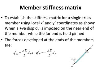
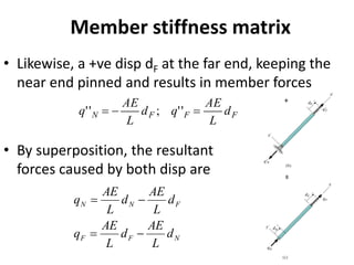
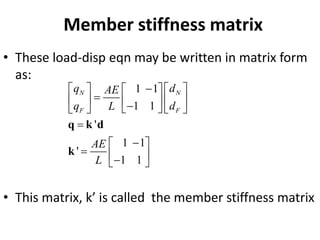
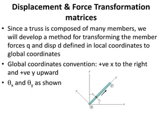
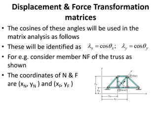
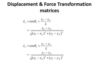
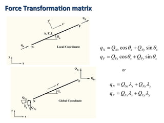
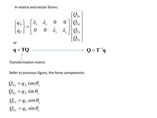
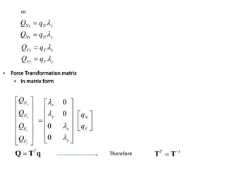
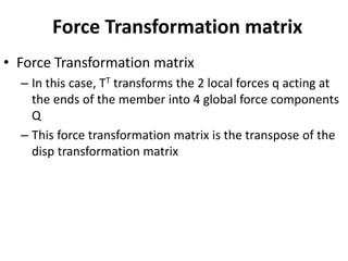
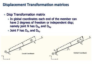
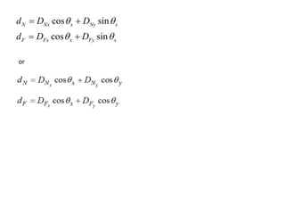
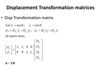
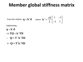
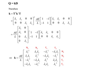
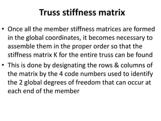
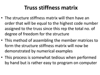
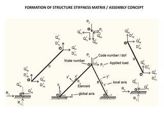
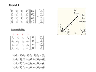
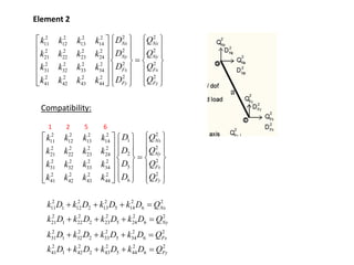
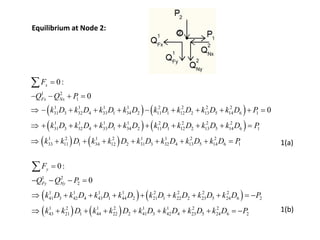
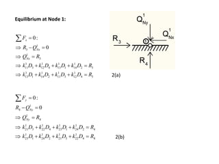
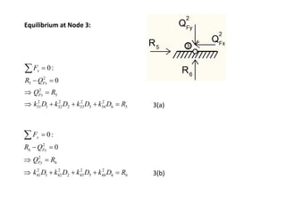
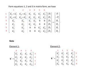
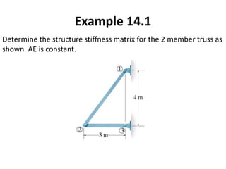
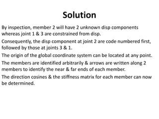
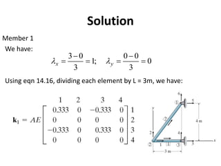
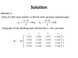
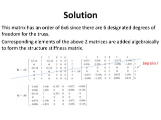
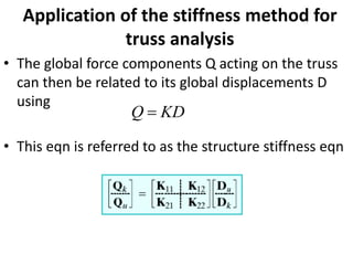
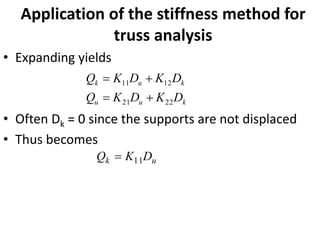
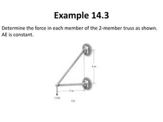
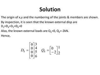
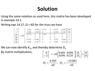
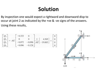
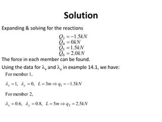
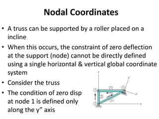
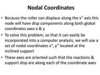
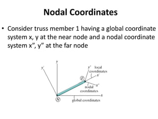
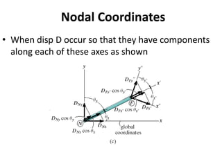
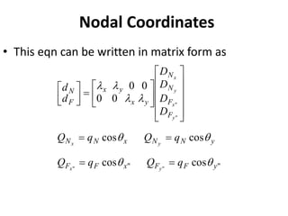
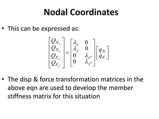
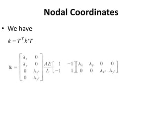
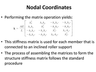
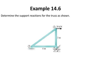
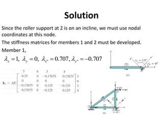
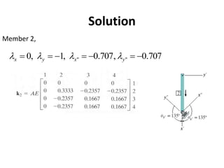
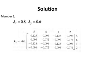
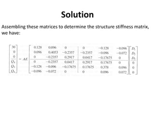
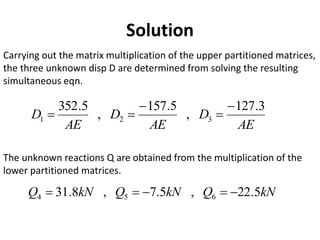
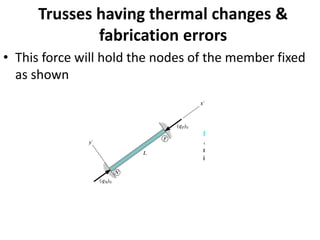
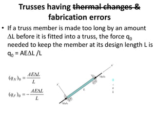
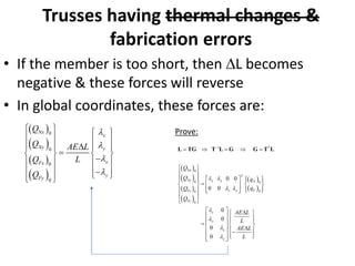
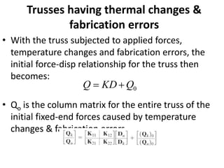
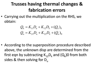
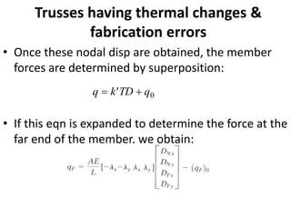
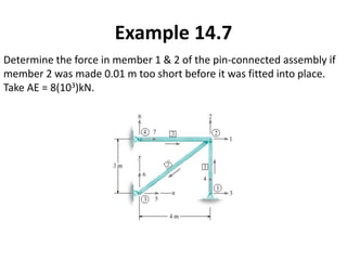
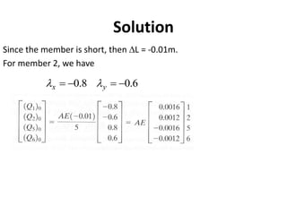
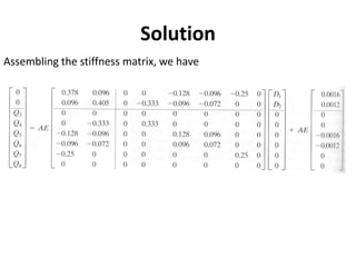
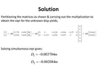
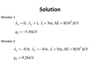
TRUSS ANALYSIS USING THE STIFFNESS METHOD
REFERENCE
STRUCTURAL ANALYSIS 7th EDITION IN SI UNITS
BY R.C. HIBBELER
Note: All this slides are just for my students
Fundamentals of the stiffness method
• The stiffness method:
– Is a disp method of analysis
– Can be used to analyse both statically determinate and
indeterminate structures
– Yields the disp & forces directly
• It is generally much easier to formulate the
necessary matrices for the computer using the
stiffness method
Fundamentals of the stiffness method
• Application of the stiffness method requires
subdividing the structure into a series of discrete
finite elements & identifying their end points as
nodes
• For truss analysis, the finite elements are
represented by each of the members that compose
the truss & the nodes represent the joints
• The force-disp properties of each element are
determined & then related to one another using the
force eqm eqn written at the nodes
Fundamentals of the stiffness method
• These relationships for the entire structure are then
grouped together into the structure stiffness matrix,
K
• The unknown disp of the nodes can then be
determined for any given loading on the structure
• When these disp are known, the external & internal
forces in the structure can be calculated using the
force-disp relations for each member
Member stiffness matrix
=
By superposition principle:
+
(a) (b)
(c)
Member stiffness matrix
• To establish the stiffness matrix for a single truss
member using local x’ and y’ coordinates as shown
When a +ve disp dN is imposed on the near end of
the member while the far end is held pinned
• The forces developed at the ends of the members
are:
N
F
N
N d
L
AE
q
d
L
AE
q −
=
= '
;
'
Member stiffness matrix
• Likewise, a +ve disp dF at the far end, keeping the
near end pinned and results in member forces
• By superposition, the resultant
forces caused by both disp are
F
F
F
N d
L
AE
q
d
L
AE
q =
−
= '
'
;
'
'
N
F
F
F
N
N
d
L
AE
d
L
AE
q
d
L
AE
d
L
AE
q
−
=
−
=
Member stiffness matrix
• These load-disp eqn may be written in matrix form
as:
• This matrix, k’ is called the member stiffness matrix
1 1
1 1
'
1 1
'
1 1
N N
F F
q d
AE
q d
L
AE
L
−
   
 
=
   
 
−
 
   
=
−
 
=  
−
 
q k d
k
Displacement & Force Transformation
matrices
• Since a truss is composed of many members, we
will develop a method for transforming the member
forces q and disp d defined in local coordinates to
global coordinates
• Global coordinates convention: +ve x to the right
and +ve y upward
• x and y as shown
Displacement & Force Transformation
matrices
• The cosines of these angles will be used in the
matrix analysis as follows
• These will be identified as
• For e.g. consider member NF of the truss as
shown
• The coordinates of N & F
are (xN, yN ) and (xF, yF )
y
y
x
x 


 cos
;
cos =
=
Displacement & Force Transformation
matrices
2
2
2
2
)
(
)
(
cos
)
(
)
(
cos
N
F
N
F
N
F
N
F
y
y
N
F
N
F
N
F
N
F
x
x
y
y
x
x
y
y
L
y
y
y
y
x
x
x
x
L
x
x
−
+
−
−
=
−
=
=
−
+
−
−
=
−
=
=




Force Transformation matrix
cos sin
cos sin
N Nx x Ny x
F Fx x Fy x
q Q Q
q Q Q
 
 
= +
= +
or
N Nx x Ny y
F Fx x Fy y
q Q Q
q Q Q
 
 
= +
= +
0 0
0 0
Nx
x y Ny
N
x y Fx
F
Fy
Q
Q
q
Q
q
Q
 
 
 
 
 
   
=
   
 
     
 
 
In matrix and vector forms:
=
q TQ
or
Transformation matrix
Refer to previous figure, the force components:
cos
sin
Nx N x
Ny N x
Q q
Q q


=
=
cos
sin
Fx F x
Fy F x
Q q
Q q


=
=
1
−
=
Q T q
or
Therefore 1
T −
=
T T
Nx N x
Ny N y
Q q
Q q


=
=
Fx F x
Fy F y
Q q
Q q


=
=
• Force Transformation matrix
• In matrix form
0
0
0
0
x
y
x
y
N x
N y N
F x F
y
F
T
Q
Q q
Q q
Q




   
   
   
 
=
   
   
   
   
 
 
=
Q T q
Force Transformation matrix
• Force Transformation matrix
– In this case, TT transforms the 2 local forces q acting at
the ends of the member into 4 global force components
Q
– This force transformation matrix is the transpose of the
disp transformation matrix
Displacement Transformation matrices
cos sin
cos sin
N Nx x Ny x
F Fx x Fy x
d D D
d D D
 
 
= +
= +
or
Displacement Transformation matrices
• Disp Transformation matrix
Let cos ; cos
;
In matrix form,
0 0
0 0
x y x y
x
y
x
y
x x y y
N N x N y F F x F y
N
N
x y
N
x y F
F
F
d D D d D D
D
D
d
D
d
D
   
   
 
 
= =
= + = +
 
 
 
   
=  
   
 
     
 
 
=
d TD
From the relation '
q k d
= where
1 1
'
1 1
AE
L
−
 
=  
−
 
k
1
'
'
'
q k d
TQ k TD
Q = T k TD
−
=
 =

Substituting:
or '
Q = T k TD
T
Member global stiffness matrix
Therefore
Q = kD
'
0 0 0 0
1 1
0 0 0 0
1 1
0
0 0 0
1 1
0 0
0 1 1
0
T
T
x y x y
x y x y
x
y x y
x y
x
y
AE
L
AE
L
   
   

  
 


=
−
   
 
=    
 
−
 
   
 
 
−  
 
 
=  
 
  −
   
 
 
 
k T k T
2 2
2 2
2 2
2 2
x x y x x y
x y y x y y
x x y x x y
x y y x y y
AE
L
     
     
     
     
 
− −
 
− −
 
 =
 
− −
 
− −
 
 
k
Nx Ny Fx Fy
Nx
Ny
Fx
Fy
Truss stiffness matrix
• Once all the member stiffness matrices are formed
in the global coordinates, it becomes necessary to
assemble them in the proper order so that the
stiffness matrix K for the entire truss can be found
• This is done by designating the rows & columns of
the matrix by the 4 code numbers used to identify
the 2 global degrees of freedom that can occur at
each end of the member
Truss stiffness matrix
• The structure stiffness matrix will then have an
order that will be equal to the highest code number
assigned to the truss since this rep the total no. of
degree of freedom for the structure
• This method of assembling the member matrices to
form the structure stiffness matrix will now be
demonstrated by numerical examples
• This process is somewhat tedious when performed
by hand but is rather easy to program on computer
FORMATION OF STRUCTURE STIFFNESS MATRIX / ASSEMBLY CONCEPT
Element 1
1 1
1 1 1 1
11 12 13 14
1 1
1 1 1 1
21 22 23 24
1 1
1 1 1 1
31 32 33 34
1 1
1 1 1 1
41 42 43 44
Nx Nx
Ny Ny
Fx Fx
Fy Fy
D Q
k k k k
D Q
k k k k
D Q
k k k k
D Q
k k k k
   
 
   
 
   
  =
   
     
     
 
     
Compatibility:
1 1 1 1 1
11 3 12 4 13 1 14 2
1 1 1 1 1
21 3 22 4 23 1 24 2
1 1 1 1 1
31 3 32 4 33 1 34 2
1 1 1 1 1
41 3 42 4 43 1 44 2
Nx
Ny
Fx
Fy
k D k D k D k D Q
k D k D k D k D Q
k D k D k D k D Q
k D k D k D k D Q
+ + + =
+ + + =
+ + + =
+ + + =
1
1 1 1 1
3
11 12 13 14
1
1 1 1 1
4
21 22 23 24
1
1 1 1 1
1
31 32 33 34
1
1 1 1 1
2
41 42 43 44
Nx
Ny
Fx
Fy
Q
D
k k k k
Q
D
k k k k
Q
D
k k k k
Q
D
k k k k
 
   
 
   
   
  =
   
     
     
   
   
3 4 1 2
Element 2
2 2
2 2 2 2
11 12 13 14
2 2
2 2 2 2
21 22 23 24
2 2
2 2 2 2
31 32 33 34
2 2
2 2 2 2
41 42 43 44
Nx Nx
Ny Ny
Fx Fx
Fy Fy
D Q
k k k k
D Q
k k k k
D Q
k k k k
D Q
k k k k
   
 
   
 
   
  =
   
     
     
 
     
Compatibility:
2 2 2 2 2
11 1 12 2 13 5 14 6
2 2 2 2 2
21 1 22 2 23 5 24 6
2 2 2 2 2
31 1 32 2 33 5 34 6
2 2 2 2 2
41 1 42 2 43 5 44 6
Nx
Ny
Fx
Fy
k D k D k D k D Q
k D k D k D k D Q
k D k D k D k D Q
k D k D k D k D Q
+ + + =
+ + + =
+ + + =
+ + + =
2
2 2 2 2
1
11 12 13 14
2
2 2 2 2
2
21 22 23 24
2
2 2 2 2
5
31 32 33 34
2
2 2 2 2
6
41 42 43 44
Nx
Ny
Fx
Fy
D Q
k k k k
D Q
k k k k
D Q
k k k k
D Q
k k k k
 
   
 
   
   
  =
   
     
     
   
   
1 2 5 6
Equilibrium at Node 2:
( ) ( )
( ) ( )
( ) ( )
1 2
1
1 1 1 1 2 2 2 2
31 3 32 4 33 1 34 2 11 1 12 2 13 5 14 6 1
1 1 1 1 2 2 2 2
31 3 32 4 33 1 34 2 11 1 12 2 13 5 14 6 1
1 2 1 2 1 1 2 2
33 11 1 34 12 2 31 3 32 4 13 5 14 6 1
0:
0
0
x
Fx Nx
F
Q Q P
k D k D k D k D k D k D k D k D P
k k D k k D k D k D k D k D P
=
− − + =
 − + + + − + + + + =
 + + + + + + + + =
 + + + + + + + =

( ) ( )
( ) ( )
1 2
2
1 1 1 1 2 2 2 2
41 3 42 4 43 1 44 2 21 1 22 2 23 5 24 6 2
1 2 1 2 1 1 2 2
43 21 1 44 22 2 41 3 42 4 23 5 24 6 2
0:
0
y
Fy Ny
F
Q Q P
k D k D k D k D k D k D k D k D P
k k D k k D k D k D k D k D P
=
− − − =
 + + + + + + + = −
 + + + + + + + = −

1(a)
1(b)
Equilibrium at Node 1:
1
3
1
3
1 1 1 1
11 3 12 4 13 1 14 2 3
1 1 1 1
13 1 14 2 11 3 12 4 3
0:
0
x
Nx
Nx
F
R Q
Q R
k D k D k D k D R
k D k D k D k D R
=
 − =
 =
 + + + =
 + + + =

1
4
1
4
1 1 1 1
21 3 22 4 23 1 24 2 4
1 1 1 1
23 1 24 2 21 3 22 4 4
0:
0
y
Ny
Ny
F
R Q
Q R
k D k D k D k D R
k D k D k D k D R
=
− =
 =
 + + + =
 + + + =

2(a)
2(b)
Equilibrium at Node 3:
2
5
2
5
2 2 2 2
31 1 32 2 33 5 34 6 5
0:
0
x
Fx
Fx
F
R Q
Q R
k D k D k D k D R
=
− =
 =
 + + + =

2
6
2
6
2 2 2 2
41 1 42 2 43 5 44 6 6
0:
0
y
Fy
Fy
F
R Q
Q R
k D k D k D k D R
=
− =
 =
 + + + =

3(a)
3(b)
Form equations 1, 2 and 3 in matrix form, we have
1 2 1 2 1 1 2 2
1 1
33 11 34 12 31 32 13 14
1 2 1 2 1 1 2 2
2 2
43 21 44 22 41 42 23 24
1 1 1 1
3
13 14 11 12
1 1 1 1
4
23 24 21 22
2 2 2 2
5
31 32 33 34
2 2 2 2
6
41 42 43 44
0 0
0 0
0 0
0 0
D P
k k k k k k k k
D P
k k k k k k k k
D
k k k k
D
k k k k
D
k k k k
D
k k k k
 
+ +  
    −
+ +
   
   
 
=
   
   
   
   
 
   
 
3
4
5
6
R
R
R
R
 
 
 
 
 
 
 
 
 
 
 
1 2 5 6
3 4
Note
1 1 1 1
11 12 13 14
1 1 1 1
1 21 22 23 24
1 1 1 1
31 32 33 34
1 1 1 1
41 42 43 44
k k k k
k k k k
k k k k
k k k k
 
 
 
=
 
 
 
 
k
3 4 1 2
Element 1:
3
4
1
2
1
2
5
6
3
4
Element 2:
2 2 2 2
11 12 13 14
2 2 2 2
2 21 22 23 24
2 2 2 2
31 32 33 34
2 2 2 2
41 42 43 44
k k k k
k k k k
k k k k
k k k k
 
 
 
=
 
 
 
 
k
1 2 5 6
1
2
5
6
Determine the structure stiffness matrix for the 2 member truss as
shown. AE is constant.
Example 14.1
By inspection, member 2 will have 2 unknown disp components
whereas joint 1 & 3 are constrained from disp.
Consequently, the disp component at joint 2 are code numbered first,
followed by those at joints 3 & 1.
The origin of the global coordinate system can be located at any point.
The members are identified arbitrarily & arrows are written along 2
members to identify the near & far ends of each member.
The direction cosines & the stiffness matrix for each member can now
be determined.
Solution
Member 1
We have:
Using eqn 14.16, dividing each element by L = 3m, we have:
Solution
0
3
0
0
;
1
3
0
3
=
−
=
=
−
= y
x 

Member 2
Since 2 is the near end & 1 is the far end, we have: (amend eqn)
Using eqn 14.16, dividing each element by L = 5m, we have:
Solution
8
.
0
5
0
4
;
6
.
0
5
0
3
=
−
=
=
−
= y
x 

This matrix has an order of 6x6 since there are 6 designated degrees of
freedom for the truss.
Corresponding elements of the above 2 matrices are added algebraically
to form the structure stiffness matrix.
Solution
Skip this !
Application of the stiffness method for
truss analysis
• The global force components Q acting on the truss
can then be related to its global displacements D
using
• This eqn is referred to as the structure stiffness eqn
KD
Q =
Application of the stiffness method for
truss analysis
• Expanding yields
• Often Dk = 0 since the supports are not displaced
• Thus becomes
u
k D
K
Q 11
=
k
u
u
k
u
k
D
K
D
K
Q
D
K
D
K
Q
22
21
12
11
+
=
+
=
Application of the stiffness method for
truss analysis
• Since the elements in the partitioned matrix K11
represent the total resistance at a truss joint to a
unit disp in either the x or y direction, then the
above eqn symbolizes the collection of all the force
eqm eqn applied to the joints where the external
loads are zero or have a known value Qk
• Solving for Du, we have:
  k
u Q
K
D
1
11
−
=
Application of the stiffness method for
truss analysis
• With Dk =0 yields
• The member forces can be determined
u
u D
K
Q 21
=
Application of the stiffness method for
truss analysis
• Since with qN = -qF for eqm,
Nx
Ny
F x y x y
Fx
Fy
D
D
AE
q
D
L
D
   
 
 
 
 
= − −  
 
 
 
 
Determine the force in each member of the 2-member truss as shown.
AE is constant.
Example 14.3
The origin of x,y and the numbering of the joints & members are shown.
By inspection, it is seen that the known external disp are
D3=D4=D5=D6=0
Also, the known external loads are Q1=0, Q2=-2kN.
Hence,
Solution
© 2009 Pearson Education South Asia Pte Ltd
Structural Analysis 7th Edition
2
1
2
0
6
5
4
3
0
0
0
0






−
=










= k
k Q
D
Using the same notation as used here, this matrix has been developed
in example 14.1.
Writing eqn 14.17, Q = KD for the truss we have
We can now identify K11 and thereby determine Du
By matrix multiplication,
Solution
D
D
.
.
.
.
AE






+












=






− 0
0
128
0
096
0
096
0
405
0
2
0
2
1
AE
D
AE
D
003
.
19
;
505
.
4
2
1
−
=
=
By inspection one would expect a rightward and downward disp to
occur at joint 2 as indicated by the +ve & -ve signs of the answers.
Using these results,
Solution
Expanding & solving for the reactions
The force in each member can be found.
Using the data for x and y in example 14.1, we have:
Solution
kN
Q
kN
Q
kN
Q
kN
Q
0
.
2
5
.
1
0
5
.
1
6
5
4
3
=
=
=
−
=
kN
q
m
L
kN
q
m
L
y
x
y
x
5
.
2
5
,
8
.
0
,
6
.
0
2,
member
For
5
.
1
3
,
0
,
1
1,
member
For
2
1
=

=
=
=
−
=

=
=
=




Nodal Coordinates
• A truss can be supported by a roller placed on a
incline
• When this occurs, the constraint of zero deflection
at the support (node) cannot be directly defined
using a single horizontal & vertical global coordinate
system
• Consider the truss
• The condition of zero disp
at node 1 is defined only
along the y” axis
Nodal Coordinates
• Because the roller can displace along the x” axis this
node will have disp components along both global
coordinates axes x & y
• To solve this problem, so that it can easily be
incorporated into a computer analysis, we will use a
set of nodal coordinates x”, y” located at the
inclined support
• These axes are oriented such that the reactions &
support disp are along each of the coordinate axes
Nodal Coordinates
• To determine the global stiffness eqn for the truss,
it becomes necessary to develop force & disp
transformation matrices for each of the connecting
members at this support so that the results can be
summed within the same global x, y coordinate
system
Nodal Coordinates
• Consider truss member 1 having a global coordinate
system x, y at the near node and a nodal coordinate
system x”, y” at the far node
Nodal Coordinates
• When disp D occur so that they have components
along each of these axes as shown
Nodal Coordinates
• This eqn can be written in matrix form as
"
" cos
cos
cos
cos
0
0
0
0
"
"
"
"
y
F
F
x
F
F
y
N
N
x
N
N
F
F
N
N
y
x
y
x
F
N
q
Q
q
Q
q
Q
q
Q
D
D
D
D
d
d
y
x
y
x
y
x
y
x








=
=
=
=


















=






Nodal Coordinates
• This can be expressed as:
• The disp & force transformation matrices in the
above eqn are used to develop the member
stiffness matrix for this situation
















=












F
N
y
x
y
x
F
F
N
N
q
q
Q
Q
Q
Q
y
x
y
x
0
0
0
0
"
"
"
"




Nodal Coordinates
• We have
T
k
T
k T
'
=
Nodal Coordinates
• Performing the matrix operation yields:
• This stiffness matrix is used for each member that is
connected to an inclined roller support
• The process of assembling the matrices to form the
structure stiffness matrix follows the standard
procedure
Determine the support reactions for the truss as shown.
Example 14.6
Since the roller support at 2 is on an incline, we must use nodal
coordinates at this node.
The stiffness matrices for members 1 and 2 must be developed.
Member 1,
Solution
707
.
0
,
707
.
0
,
0
,
1 "
" −
=
=
=
= y
x
y
x 



Member 2,
Solution
707
.
0
,
707
.
0
,
1
,
0 "
" −
=
−
=
−
=
= y
x
y
x 



Member 3,
Solution
6
.
0
,
8
.
0 =
= y
x 

Assembling these matrices to determine the structure stiffness matrix,
we have:
Solution
Carrying out the matrix multiplication of the upper partitioned matrices,
the three unknown disp D are determined from solving the resulting
simultaneous eqn.
The unknown reactions Q are obtained from the multiplication of the
lower partitioned matrices.
Solution
AE
D
AE
D
AE
D
3
.
127
,
5
.
157
,
5
.
352
3
2
1
−
=
−
=
=
kN
Q
kN
Q
kN
Q 5
.
22
,
5
.
7
,
8
.
31 6
5
4 −
=
−
=
=
Trusses having thermal changes &
fabrication errors
• If some of the members of the truss are subjected
to an increase or decrease in length due to thermal
changes or fabrication errors, then it is necessary to
use the method of superposition to obtain the
solution
• This requires 3 steps
Trusses having thermal changes &
fabrication errors
• First, the fixed end forces necessary to prevent
movement of the nodes as caused by temperature
or fabrication are calculated
• Second, equal but opposite forces are placed on the
truss at the nodes & the disp of the nodes are
calculated using the matrix analysis
• Third, the actual forces in the members & the
reactions on the truss are determined by
superposing these 2 results
Trusses having thermal changes &
fabrication errors
• This force will hold the nodes of the member fixed
as shown
Trusses having thermal changes &
fabrication errors
• This procedure is only necessary if the truss is
statically indeterminate
• If a truss member of length L is subjected to a
temperature increase T, the member will undergo
an increase in length of L =  TL
• A compressive force q0 applied to the member will
cause a decrease in the member’s length of L’ =
q0L/AE
• If we equate these 2 disp q0 = AE T
Trusses having thermal changes &
fabrication errors
• This force will hold the nodes of the member fixed
as shown in the figure
• If a temperature decrease occurs then T becomes
negative & these forces reverse direction to hold
the member in eqm
T
AE
q
T
AE
q
F
N

−
=

=


0
0
)
(
)
(
Trusses having thermal changes &
fabrication errors
• If a truss member is made too long by an amount
L before it is fitted into a truss, the force q0
needed to keep the member at its design length L is
q0 = AEL /L
L
L
AE
q
L
L
AE
q
F
N

−
=

=
0
0
)
(
)
(
Trusses having thermal changes &
fabrication errors
• If the member is too short, then L becomes
negative & these forces will reverse
• In global coordinates, these forces are:
Prove:
( )
( )
( )
( )
( )
( )
1
0
0 0
0
0
0
0 0
0 0
0
0
0
0
T
Nx
T
Ny x y N
F
x y
Fx
Fy
x
y
x
y
Q
Q q
q
Q
Q
AE L
L
AE L
L
 
 




−
=  =  =
 
 
   
   
=  
   
 
   
   
 
 
  
 
   
 
 
=  
  
 
−
   
 
 
 
L TG T L G G T L
( )
( )
( )
( )
0
0
0
0
Nx
x
Ny y
x
Fx
y
Fy
Q
Q AE L
L
Q
Q




   
   
    
=
   
−
   
   
−
 
 
Trusses having thermal changes &
fabrication errors
• With the truss subjected to applied forces,
temperature changes and fabrication errors, the
initial force-disp relationship for the truss then
becomes:
• Qo is the column matrix for the entire truss of the
initial fixed-end forces caused by temperature
changes & fabrication errors
0
Q
KD
Q +
=
Trusses having thermal changes &
fabrication errors
• Carrying out the multiplication on the RHS, we
obtain:
• According to the superposition procedure described
above, the unknown disp are determined from the
first eqn by subtracting K12Dk and (Qk)0 from both
sides & then solving for Du
0
22
21
0
12
11
)
(
)
(
u
k
u
u
k
k
u
k
Q
D
K
D
K
Q
Q
D
K
D
K
Q
+
+
=
+
+
=
Trusses having thermal changes &
fabrication errors
• Once these nodal disp are obtained, the member
forces are determined by superposition:
• If this eqn is expanded to determine the force at the
far end of the member, we obtain:
0
' q
TD
k
q +
=
Determine the force in member 1 & 2 of the pin-connected assembly if
member 2 was made 0.01 m too short before it was fitted into place.
Take AE = 8(103)kN.
Example 14.7
Since the member is short, then L = -0.01m.
For member 2, we have
Solution
6
.
0
8
.
0 −
=
−
= y
x 

Assembling the stiffness matrix, we have
Solution
Partitioning the matrices as shown & carrying out the multiplication to
obtain the eqn for the unknown disp yields,
Solving simultaneous eqn gives:
Solution
m
D
m
D
002084
.
0
003704
.
0
2
1
−
=
−
=
Member 1
Member 2
Solution
kN
q
kN
L
y
x
56
.
5
)
10
(
8
AE
,
3m
,
1
,
0
1
3
−
=
=
=
=
= 

kN
q
kN
L
y
x
26
.
9
)
10
(
8
AE
,
5m
,
6
.
0
,
8
.
0
2
3
=
=
=
−
=
−
= 


Stiffness Method for structure analysis - Truss

  • 1.
    TRUSS ANALYSIS USINGTHE STIFFNESS METHOD REFERENCE STRUCTURAL ANALYSIS 7th EDITION IN SI UNITS BY R.C. HIBBELER Note: All this slides are just for my students
  • 2.
    Fundamentals of thestiffness method • The stiffness method: – Is a disp method of analysis – Can be used to analyse both statically determinate and indeterminate structures – Yields the disp & forces directly • It is generally much easier to formulate the necessary matrices for the computer using the stiffness method
  • 3.
    Fundamentals of thestiffness method • Application of the stiffness method requires subdividing the structure into a series of discrete finite elements & identifying their end points as nodes • For truss analysis, the finite elements are represented by each of the members that compose the truss & the nodes represent the joints • The force-disp properties of each element are determined & then related to one another using the force eqm eqn written at the nodes
  • 4.
    Fundamentals of thestiffness method • These relationships for the entire structure are then grouped together into the structure stiffness matrix, K • The unknown disp of the nodes can then be determined for any given loading on the structure • When these disp are known, the external & internal forces in the structure can be calculated using the force-disp relations for each member
  • 5.
    Member stiffness matrix = Bysuperposition principle: + (a) (b) (c)
  • 6.
    Member stiffness matrix •To establish the stiffness matrix for a single truss member using local x’ and y’ coordinates as shown When a +ve disp dN is imposed on the near end of the member while the far end is held pinned • The forces developed at the ends of the members are: N F N N d L AE q d L AE q − = = ' ; '
  • 7.
    Member stiffness matrix •Likewise, a +ve disp dF at the far end, keeping the near end pinned and results in member forces • By superposition, the resultant forces caused by both disp are F F F N d L AE q d L AE q = − = ' ' ; ' ' N F F F N N d L AE d L AE q d L AE d L AE q − = − =
  • 8.
    Member stiffness matrix •These load-disp eqn may be written in matrix form as: • This matrix, k’ is called the member stiffness matrix 1 1 1 1 ' 1 1 ' 1 1 N N F F q d AE q d L AE L −       =       −       = −   =   −   q k d k
  • 9.
    Displacement & ForceTransformation matrices • Since a truss is composed of many members, we will develop a method for transforming the member forces q and disp d defined in local coordinates to global coordinates • Global coordinates convention: +ve x to the right and +ve y upward • x and y as shown
  • 10.
    Displacement & ForceTransformation matrices • The cosines of these angles will be used in the matrix analysis as follows • These will be identified as • For e.g. consider member NF of the truss as shown • The coordinates of N & F are (xN, yN ) and (xF, yF ) y y x x     cos ; cos = =
  • 11.
    Displacement & ForceTransformation matrices 2 2 2 2 ) ( ) ( cos ) ( ) ( cos N F N F N F N F y y N F N F N F N F x x y y x x y y L y y y y x x x x L x x − + − − = − = = − + − − = − = =    
  • 12.
    Force Transformation matrix cossin cos sin N Nx x Ny x F Fx x Fy x q Q Q q Q Q     = + = + or N Nx x Ny y F Fx x Fy y q Q Q q Q Q     = + = +
  • 13.
    0 0 0 0 Nx xy Ny N x y Fx F Fy Q Q q Q q Q               =                 In matrix and vector forms: = q TQ or Transformation matrix Refer to previous figure, the force components: cos sin Nx N x Ny N x Q q Q q   = = cos sin Fx F x Fy F x Q q Q q   = = 1 − = Q T q
  • 14.
    or Therefore 1 T − = TT Nx N x Ny N y Q q Q q   = = Fx F x Fy F y Q q Q q   = = • Force Transformation matrix • In matrix form 0 0 0 0 x y x y N x N y N F x F y F T Q Q q Q q Q                   =                     = Q T q
  • 15.
    Force Transformation matrix •Force Transformation matrix – In this case, TT transforms the 2 local forces q acting at the ends of the member into 4 global force components Q – This force transformation matrix is the transpose of the disp transformation matrix
  • 16.
  • 17.
    cos sin cos sin NNx x Ny x F Fx x Fy x d D D d D D     = + = + or
  • 18.
    Displacement Transformation matrices •Disp Transformation matrix Let cos ; cos ; In matrix form, 0 0 0 0 x y x y x y x y x x y y N N x N y F F x F y N N x y N x y F F F d D D d D D D D d D d D             = = = + = +           =                   = d TD
  • 19.
    From the relation' q k d = where 1 1 ' 1 1 AE L −   =   −   k 1 ' ' ' q k d TQ k TD Q = T k TD − =  =  Substituting: or ' Q = T k TD T Member global stiffness matrix
  • 20.
    Therefore Q = kD ' 00 0 0 1 1 0 0 0 0 1 1 0 0 0 0 1 1 0 0 0 1 1 0 T T x y x y x y x y x y x y x y x y AE L AE L                 = −       =       −           −       =       −           k T k T 2 2 2 2 2 2 2 2 x x y x x y x y y x y y x x y x x y x y y x y y AE L                           − −   − −    =   − −   − −     k Nx Ny Fx Fy Nx Ny Fx Fy
  • 21.
    Truss stiffness matrix •Once all the member stiffness matrices are formed in the global coordinates, it becomes necessary to assemble them in the proper order so that the stiffness matrix K for the entire truss can be found • This is done by designating the rows & columns of the matrix by the 4 code numbers used to identify the 2 global degrees of freedom that can occur at each end of the member
  • 22.
    Truss stiffness matrix •The structure stiffness matrix will then have an order that will be equal to the highest code number assigned to the truss since this rep the total no. of degree of freedom for the structure • This method of assembling the member matrices to form the structure stiffness matrix will now be demonstrated by numerical examples • This process is somewhat tedious when performed by hand but is rather easy to program on computer
  • 23.
    FORMATION OF STRUCTURESTIFFNESS MATRIX / ASSEMBLY CONCEPT
  • 24.
    Element 1 1 1 11 1 1 11 12 13 14 1 1 1 1 1 1 21 22 23 24 1 1 1 1 1 1 31 32 33 34 1 1 1 1 1 1 41 42 43 44 Nx Nx Ny Ny Fx Fx Fy Fy D Q k k k k D Q k k k k D Q k k k k D Q k k k k                   =                         Compatibility: 1 1 1 1 1 11 3 12 4 13 1 14 2 1 1 1 1 1 21 3 22 4 23 1 24 2 1 1 1 1 1 31 3 32 4 33 1 34 2 1 1 1 1 1 41 3 42 4 43 1 44 2 Nx Ny Fx Fy k D k D k D k D Q k D k D k D k D Q k D k D k D k D Q k D k D k D k D Q + + + = + + + = + + + = + + + = 1 1 1 1 1 3 11 12 13 14 1 1 1 1 1 4 21 22 23 24 1 1 1 1 1 1 31 32 33 34 1 1 1 1 1 2 41 42 43 44 Nx Ny Fx Fy Q D k k k k Q D k k k k Q D k k k k Q D k k k k                   =                         3 4 1 2
  • 25.
    Element 2 2 2 22 2 2 11 12 13 14 2 2 2 2 2 2 21 22 23 24 2 2 2 2 2 2 31 32 33 34 2 2 2 2 2 2 41 42 43 44 Nx Nx Ny Ny Fx Fx Fy Fy D Q k k k k D Q k k k k D Q k k k k D Q k k k k                   =                         Compatibility: 2 2 2 2 2 11 1 12 2 13 5 14 6 2 2 2 2 2 21 1 22 2 23 5 24 6 2 2 2 2 2 31 1 32 2 33 5 34 6 2 2 2 2 2 41 1 42 2 43 5 44 6 Nx Ny Fx Fy k D k D k D k D Q k D k D k D k D Q k D k D k D k D Q k D k D k D k D Q + + + = + + + = + + + = + + + = 2 2 2 2 2 1 11 12 13 14 2 2 2 2 2 2 21 22 23 24 2 2 2 2 2 5 31 32 33 34 2 2 2 2 2 6 41 42 43 44 Nx Ny Fx Fy D Q k k k k D Q k k k k D Q k k k k D Q k k k k                   =                         1 2 5 6
  • 26.
    Equilibrium at Node2: ( ) ( ) ( ) ( ) ( ) ( ) 1 2 1 1 1 1 1 2 2 2 2 31 3 32 4 33 1 34 2 11 1 12 2 13 5 14 6 1 1 1 1 1 2 2 2 2 31 3 32 4 33 1 34 2 11 1 12 2 13 5 14 6 1 1 2 1 2 1 1 2 2 33 11 1 34 12 2 31 3 32 4 13 5 14 6 1 0: 0 0 x Fx Nx F Q Q P k D k D k D k D k D k D k D k D P k D k D k D k D k D k D k D k D P k k D k k D k D k D k D k D P = − − + =  − + + + − + + + + =  + + + + + + + + =  + + + + + + + =  ( ) ( ) ( ) ( ) 1 2 2 1 1 1 1 2 2 2 2 41 3 42 4 43 1 44 2 21 1 22 2 23 5 24 6 2 1 2 1 2 1 1 2 2 43 21 1 44 22 2 41 3 42 4 23 5 24 6 2 0: 0 y Fy Ny F Q Q P k D k D k D k D k D k D k D k D P k k D k k D k D k D k D k D P = − − − =  + + + + + + + = −  + + + + + + + = −  1(a) 1(b)
  • 27.
    Equilibrium at Node1: 1 3 1 3 1 1 1 1 11 3 12 4 13 1 14 2 3 1 1 1 1 13 1 14 2 11 3 12 4 3 0: 0 x Nx Nx F R Q Q R k D k D k D k D R k D k D k D k D R =  − =  =  + + + =  + + + =  1 4 1 4 1 1 1 1 21 3 22 4 23 1 24 2 4 1 1 1 1 23 1 24 2 21 3 22 4 4 0: 0 y Ny Ny F R Q Q R k D k D k D k D R k D k D k D k D R = − =  =  + + + =  + + + =  2(a) 2(b)
  • 28.
    Equilibrium at Node3: 2 5 2 5 2 2 2 2 31 1 32 2 33 5 34 6 5 0: 0 x Fx Fx F R Q Q R k D k D k D k D R = − =  =  + + + =  2 6 2 6 2 2 2 2 41 1 42 2 43 5 44 6 6 0: 0 y Fy Fy F R Q Q R k D k D k D k D R = − =  =  + + + =  3(a) 3(b)
  • 29.
    Form equations 1,2 and 3 in matrix form, we have 1 2 1 2 1 1 2 2 1 1 33 11 34 12 31 32 13 14 1 2 1 2 1 1 2 2 2 2 43 21 44 22 41 42 23 24 1 1 1 1 3 13 14 11 12 1 1 1 1 4 23 24 21 22 2 2 2 2 5 31 32 33 34 2 2 2 2 6 41 42 43 44 0 0 0 0 0 0 0 0 D P k k k k k k k k D P k k k k k k k k D k k k k D k k k k D k k k k D k k k k   + +       − + +           =                         3 4 5 6 R R R R                       1 2 5 6 3 4 Note 1 1 1 1 11 12 13 14 1 1 1 1 1 21 22 23 24 1 1 1 1 31 32 33 34 1 1 1 1 41 42 43 44 k k k k k k k k k k k k k k k k       =         k 3 4 1 2 Element 1: 3 4 1 2 1 2 5 6 3 4 Element 2: 2 2 2 2 11 12 13 14 2 2 2 2 2 21 22 23 24 2 2 2 2 31 32 33 34 2 2 2 2 41 42 43 44 k k k k k k k k k k k k k k k k       =         k 1 2 5 6 1 2 5 6
  • 30.
    Determine the structurestiffness matrix for the 2 member truss as shown. AE is constant. Example 14.1
  • 31.
    By inspection, member2 will have 2 unknown disp components whereas joint 1 & 3 are constrained from disp. Consequently, the disp component at joint 2 are code numbered first, followed by those at joints 3 & 1. The origin of the global coordinate system can be located at any point. The members are identified arbitrarily & arrows are written along 2 members to identify the near & far ends of each member. The direction cosines & the stiffness matrix for each member can now be determined. Solution
  • 32.
    Member 1 We have: Usingeqn 14.16, dividing each element by L = 3m, we have: Solution 0 3 0 0 ; 1 3 0 3 = − = = − = y x  
  • 33.
    Member 2 Since 2is the near end & 1 is the far end, we have: (amend eqn) Using eqn 14.16, dividing each element by L = 5m, we have: Solution 8 . 0 5 0 4 ; 6 . 0 5 0 3 = − = = − = y x  
  • 34.
    This matrix hasan order of 6x6 since there are 6 designated degrees of freedom for the truss. Corresponding elements of the above 2 matrices are added algebraically to form the structure stiffness matrix. Solution Skip this !
  • 35.
    Application of thestiffness method for truss analysis • The global force components Q acting on the truss can then be related to its global displacements D using • This eqn is referred to as the structure stiffness eqn KD Q =
  • 36.
    Application of thestiffness method for truss analysis • Expanding yields • Often Dk = 0 since the supports are not displaced • Thus becomes u k D K Q 11 = k u u k u k D K D K Q D K D K Q 22 21 12 11 + = + =
  • 37.
    Application of thestiffness method for truss analysis • Since the elements in the partitioned matrix K11 represent the total resistance at a truss joint to a unit disp in either the x or y direction, then the above eqn symbolizes the collection of all the force eqm eqn applied to the joints where the external loads are zero or have a known value Qk • Solving for Du, we have:   k u Q K D 1 11 − =
  • 38.
    Application of thestiffness method for truss analysis • With Dk =0 yields • The member forces can be determined u u D K Q 21 =
  • 39.
    Application of thestiffness method for truss analysis • Since with qN = -qF for eqm, Nx Ny F x y x y Fx Fy D D AE q D L D             = − −          
  • 40.
    Determine the forcein each member of the 2-member truss as shown. AE is constant. Example 14.3
  • 41.
    The origin ofx,y and the numbering of the joints & members are shown. By inspection, it is seen that the known external disp are D3=D4=D5=D6=0 Also, the known external loads are Q1=0, Q2=-2kN. Hence, Solution © 2009 Pearson Education South Asia Pte Ltd Structural Analysis 7th Edition 2 1 2 0 6 5 4 3 0 0 0 0       − =           = k k Q D
  • 42.
    Using the samenotation as used here, this matrix has been developed in example 14.1. Writing eqn 14.17, Q = KD for the truss we have We can now identify K11 and thereby determine Du By matrix multiplication, Solution D D . . . . AE       +             =       − 0 0 128 0 096 0 096 0 405 0 2 0 2 1 AE D AE D 003 . 19 ; 505 . 4 2 1 − = =
  • 43.
    By inspection onewould expect a rightward and downward disp to occur at joint 2 as indicated by the +ve & -ve signs of the answers. Using these results, Solution
  • 44.
    Expanding & solvingfor the reactions The force in each member can be found. Using the data for x and y in example 14.1, we have: Solution kN Q kN Q kN Q kN Q 0 . 2 5 . 1 0 5 . 1 6 5 4 3 = = = − = kN q m L kN q m L y x y x 5 . 2 5 , 8 . 0 , 6 . 0 2, member For 5 . 1 3 , 0 , 1 1, member For 2 1 =  = = = − =  = = =    
  • 45.
    Nodal Coordinates • Atruss can be supported by a roller placed on a incline • When this occurs, the constraint of zero deflection at the support (node) cannot be directly defined using a single horizontal & vertical global coordinate system • Consider the truss • The condition of zero disp at node 1 is defined only along the y” axis
  • 46.
    Nodal Coordinates • Becausethe roller can displace along the x” axis this node will have disp components along both global coordinates axes x & y • To solve this problem, so that it can easily be incorporated into a computer analysis, we will use a set of nodal coordinates x”, y” located at the inclined support • These axes are oriented such that the reactions & support disp are along each of the coordinate axes
  • 47.
    Nodal Coordinates • Todetermine the global stiffness eqn for the truss, it becomes necessary to develop force & disp transformation matrices for each of the connecting members at this support so that the results can be summed within the same global x, y coordinate system
  • 48.
    Nodal Coordinates • Considertruss member 1 having a global coordinate system x, y at the near node and a nodal coordinate system x”, y” at the far node
  • 49.
    Nodal Coordinates • Whendisp D occur so that they have components along each of these axes as shown
  • 50.
    Nodal Coordinates • Thiseqn can be written in matrix form as " " cos cos cos cos 0 0 0 0 " " " " y F F x F F y N N x N N F F N N y x y x F N q Q q Q q Q q Q D D D D d d y x y x y x y x         = = = =                   =      
  • 51.
    Nodal Coordinates • Thiscan be expressed as: • The disp & force transformation matrices in the above eqn are used to develop the member stiffness matrix for this situation                 =             F N y x y x F F N N q q Q Q Q Q y x y x 0 0 0 0 " " " "    
  • 52.
    Nodal Coordinates • Wehave T k T k T ' =
  • 53.
    Nodal Coordinates • Performingthe matrix operation yields: • This stiffness matrix is used for each member that is connected to an inclined roller support • The process of assembling the matrices to form the structure stiffness matrix follows the standard procedure
  • 54.
    Determine the supportreactions for the truss as shown. Example 14.6
  • 55.
    Since the rollersupport at 2 is on an incline, we must use nodal coordinates at this node. The stiffness matrices for members 1 and 2 must be developed. Member 1, Solution 707 . 0 , 707 . 0 , 0 , 1 " " − = = = = y x y x    
  • 56.
    Member 2, Solution 707 . 0 , 707 . 0 , 1 , 0 " "− = − = − = = y x y x    
  • 57.
  • 58.
    Assembling these matricesto determine the structure stiffness matrix, we have: Solution
  • 59.
    Carrying out thematrix multiplication of the upper partitioned matrices, the three unknown disp D are determined from solving the resulting simultaneous eqn. The unknown reactions Q are obtained from the multiplication of the lower partitioned matrices. Solution AE D AE D AE D 3 . 127 , 5 . 157 , 5 . 352 3 2 1 − = − = = kN Q kN Q kN Q 5 . 22 , 5 . 7 , 8 . 31 6 5 4 − = − = =
  • 60.
    Trusses having thermalchanges & fabrication errors • If some of the members of the truss are subjected to an increase or decrease in length due to thermal changes or fabrication errors, then it is necessary to use the method of superposition to obtain the solution • This requires 3 steps
  • 61.
    Trusses having thermalchanges & fabrication errors • First, the fixed end forces necessary to prevent movement of the nodes as caused by temperature or fabrication are calculated • Second, equal but opposite forces are placed on the truss at the nodes & the disp of the nodes are calculated using the matrix analysis • Third, the actual forces in the members & the reactions on the truss are determined by superposing these 2 results
  • 62.
    Trusses having thermalchanges & fabrication errors • This force will hold the nodes of the member fixed as shown
  • 63.
    Trusses having thermalchanges & fabrication errors • This procedure is only necessary if the truss is statically indeterminate • If a truss member of length L is subjected to a temperature increase T, the member will undergo an increase in length of L =  TL • A compressive force q0 applied to the member will cause a decrease in the member’s length of L’ = q0L/AE • If we equate these 2 disp q0 = AE T
  • 64.
    Trusses having thermalchanges & fabrication errors • This force will hold the nodes of the member fixed as shown in the figure • If a temperature decrease occurs then T becomes negative & these forces reverse direction to hold the member in eqm T AE q T AE q F N  − =  =   0 0 ) ( ) (
  • 65.
    Trusses having thermalchanges & fabrication errors • If a truss member is made too long by an amount L before it is fitted into a truss, the force q0 needed to keep the member at its design length L is q0 = AEL /L L L AE q L L AE q F N  − =  = 0 0 ) ( ) (
  • 66.
    Trusses having thermalchanges & fabrication errors • If the member is too short, then L becomes negative & these forces will reverse • In global coordinates, these forces are: Prove: ( ) ( ) ( ) ( ) ( ) ( ) 1 0 0 0 0 0 0 0 0 0 0 0 0 0 0 T Nx T Ny x y N F x y Fx Fy x y x y Q Q q q Q Q AE L L AE L L         − =  =  =             =                                  =        −           L TG T L G G T L ( ) ( ) ( ) ( ) 0 0 0 0 Nx x Ny y x Fx y Fy Q Q AE L L Q Q                  =     −         −    
  • 67.
    Trusses having thermalchanges & fabrication errors • With the truss subjected to applied forces, temperature changes and fabrication errors, the initial force-disp relationship for the truss then becomes: • Qo is the column matrix for the entire truss of the initial fixed-end forces caused by temperature changes & fabrication errors 0 Q KD Q + =
  • 68.
    Trusses having thermalchanges & fabrication errors • Carrying out the multiplication on the RHS, we obtain: • According to the superposition procedure described above, the unknown disp are determined from the first eqn by subtracting K12Dk and (Qk)0 from both sides & then solving for Du 0 22 21 0 12 11 ) ( ) ( u k u u k k u k Q D K D K Q Q D K D K Q + + = + + =
  • 69.
    Trusses having thermalchanges & fabrication errors • Once these nodal disp are obtained, the member forces are determined by superposition: • If this eqn is expanded to determine the force at the far end of the member, we obtain: 0 ' q TD k q + =
  • 70.
    Determine the forcein member 1 & 2 of the pin-connected assembly if member 2 was made 0.01 m too short before it was fitted into place. Take AE = 8(103)kN. Example 14.7
  • 71.
    Since the memberis short, then L = -0.01m. For member 2, we have Solution 6 . 0 8 . 0 − = − = y x  
  • 72.
    Assembling the stiffnessmatrix, we have Solution
  • 73.
    Partitioning the matricesas shown & carrying out the multiplication to obtain the eqn for the unknown disp yields, Solving simultaneous eqn gives: Solution m D m D 002084 . 0 003704 . 0 2 1 − = − =
  • 74.
    Member 1 Member 2 Solution kN q kN L y x 56 . 5 ) 10 ( 8 AE , 3m , 1 , 0 1 3 − = = = = =  kN q kN L y x 26 . 9 ) 10 ( 8 AE , 5m , 6 . 0 , 8 . 0 2 3 = = = − = − =  