BY using various models to predict the weather . Nowadays various methods have been implemented for weather forecasting.

1. SUBMITTED BY:
SOURAV KUMAR MUND
IT134672
1301209266
NUMERICAL
WEATHER
PREDICTION

2. CONTENTS
• Introduction

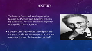
3. INTRODUCTION
• Numerical weather prediction uses mathematical models of the
atmosphere and oceans to predict the weather based on current
weather conditions .
• It produce realistic results .
• A number of global and regional forecast models are run in different
countries worldwide.
• It is relayed on radiosonde , weather satellite .

4. HISTORY
• The history of numerical weather prediction
began in the 1920s through the efforts of Lewis
Fry Richardson, who used procedures originally
developed by Vilhelm Bjerknes .
• It was not until the advent of the computer and
computer simulations that computation time was
reduced to less than the forecast period itself.

5. INITIALIZATION
• The process of entering observation data into the model to generate
initial conditions is called initialization.
• On land, terrain maps available at resolutions down to 1 kilometre(0.6
mi) globally are used to help model atmospheric circulations within
regions of rugged topography, in order to better depict features such
as downslope winds, mountain waves and related cloudiness that
affects incoming solar radiation.
• The main inputs from weather services are observations from devices
(called radiosondes) in weather balloons that measure various
atmospheric parameters and transmits them to a fixed receiver.
Weather reconnaissance aircraft

6. COMPUTATION
• An atmospheric model is a computer program that produces meteorological information for future times
at given locations and altitudes.
• Model is a set of equations, known as the primitive equations, used to predict the future state of the
atmosphere.
• These equations along with the ideal gas law are used to evolve the density, pressure, and potential
temperature scalar fields and the air velocity (wind) vector field of the atmosphere through time.
• some global models and almost all regional models use finite difference methods for all three spatial
dimensions, while other global models and a few regional models use spectral methods for the horizontal
dimensions and finite difference methods in the vertical.

7. PARAMETERIZATION
• Parameterization is a procedure for representing these processes by relating them to
variables on the scales that the model resolves.
• A typical cloud has a scale of less than 1 kilometre (0.6 mi), and would require a
grid even finer than this to be represented physically by the equations of fluid motion
the processes that such clouds represent are parameterized, by processes of various
sophistication.

8. DOMAINS
• The horizontal domain of a model is either global, covering the entire Earth, or regional,
covering only part of the Earth.
• Regional models (also known as limited area model) allow for the use of finer grid spacing
than global models because the available computational resources are focused on a specific
area instead of being spread over the globe.
• This allows regional models to resolve explicitly smaller scale meteorological phenomena
that cannot be represented on the coarser grid of a global model.
• Regional models use a global model to specify conditions at the edge of their domain
(boundary conditions) in order to allow systems from outside the regional model domain to
move into its area.

9. Horizontal coordinates
• Horizontal position may be expressed directly in geographic coordinates (latitude and longitude) for
global models or in a map projection planar coordinates for regional models.
Vertical coordinates
• The vertical coordinate is handled in various ways. Lewis Fry Richardson's 1922 model used geometric
height ( Z ) as the vertical coordinate.
• Models substituted the geometric coordinate with a pressure coordinate system, in which the
geopotential heights of constant pressure surfaces become dependent variables, greatly simplifying
the primitive equations.
• This correlation between coordinate systems can be made since pressure decreases with height
through the Earth's atmosphere.
COORDINATE SYSTEMS

10. COORDINATE SYSTEMS
Vertical coordinates
• The first model used for operational forecasts, the single layer bar tropic model, used a single pressure
coordinate at the 500millibar (about 5,500 m (18,000 ft.) level,[3] and thus was essentially two-
dimensional.
• High resolution models—also called mesoscale models such as the Weather Research and Forecasting
model tend to use normalized pressure coordinates referred to as sigma coordinates.

11. APLICATION
1. Air quality modelling
2. Climate Modelling
3. Tropical Cycle Forecasting
4. Wild Fire Modelling

12. Air Quality Modelling
• Air quality forecasting attempts to predict when the concentrations of pollutants will attain levels that are hazardous to
public health.
• The concentration of pollutants in the atmosphere is determined by their transport, or mean velocity of movement
through the atmosphere, their diffusion, chemical transformation, and ground deposition. In addition to pollutant source
and terrain information, these models require data about the state of the fluid flow in the atmosphere to determine its
transport and diffusion.
• Urban air quality models require a very fine computational mesh, requiring the use of high resolution mesoscale
weather models.
Climate modelling
• The transfer of energy between the wind blowing over the
surface of an ocean and the ocean's upper layer is an important
element in wave dynamics
• The spectral wave transport equation is used to describe the change in
wave spectrum over changing topography.

13. Tropical cyclone forecasting
• Tropical cyclone forecasting also relies on data provided by numerical weather models. Three main classes of tropical
cyclone guidance models exist: Statistical models are based on an analysis of storm behaviour using climatology, and
correlate a storm's position and date to produce a forecast that is not based on the physics of the atmosphere at the time.
Dynamical models are numerical models that solve the governing equations of fluid flow in the atmosphere; they are
based on the same principles as other limited area.
• Numerical weather prediction models but may include special computational techniques such as refined spatial domains
that move along with the cyclone. Models that use elements of both approaches are called statistical dynamical models.
• Wildfire modelling
• On a molecular scale, there are two main competing reaction processes involved in the degradation of cellulose,
or wood fuels, in wildfires.

14. REFERENCES
• 1. Lynch, Peter (March 2008). "The origins of computer weather prediction and climate modeling"
(PDF). Journal of Computational Physics. University of Miami. 227 (7): 3431–44.
Bibcode:2008JCoPh.227.3431L.doi:10.1016/j.jcp.2007.02.034. Retrieved 20101223.
• 2. Lynch, Peter (2006). "Weather Prediction by Numerical Process". The Emergence of Numerical
Weather Prediction.
• Cambridge University Press. pp. 1–27. ISBN 9780521857291.
• Wikipedia