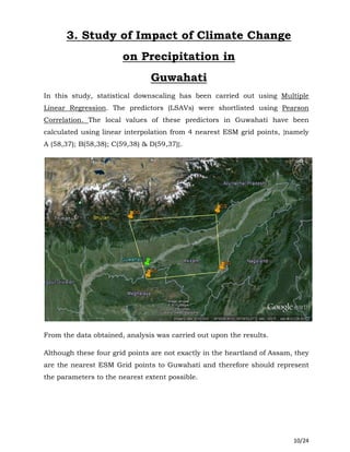
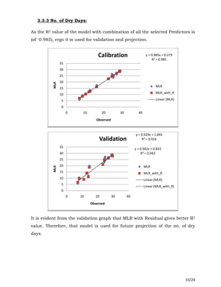
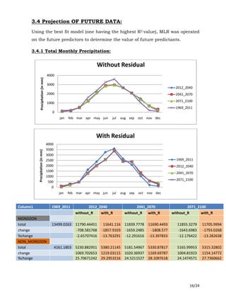
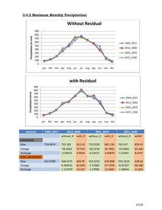
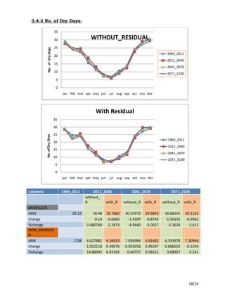
This document discusses a study analyzing the impact of climate change on precipitation characteristics in Guwahati, India using an Earth System Model. It summarizes the use of statistical downscaling with multiple linear regression to project future precipitation data. Predictors with the highest correlation to total monthly precipitation, maximum monthly precipitation, and number of dry days were selected from the ESM dataset. The downscaled results will be used for flood frequency analysis to project precipitation levels and dry days under different return periods.
1) CGCMs are coupled general circulation models that combine atmospheric and oceanic GCMs to allow the lower boundary conditions of the atmosphere to be determined interactively by ocean processes.
2) CGCM3.1 is a third generation CGCM developed by CCCMA that runs at T47 and T63 resolutions with ocean grids of roughly 1.4x0.9 degrees and 1.85 degrees respectively.
3) A study assessed CGCM3.1's wind fields in the Persian Gulf, finding it generally underestimated wind speeds compared to ECMWF reanalysis data.
General circulation models (GCMs) are computer models that simulate the operation of the climate system. GCMs take into account factors like greenhouse gases, landforms, ocean currents, and their interactions. GCMs are used to both identify possible causes of climate change and predict future climate. Contemporary GCMs are complex, three-dimensional models with thousands of individual cells that simulate atmospheric and oceanic processes globally. GCMs are the best tools available for determining the potential impacts of climate change and informing conservation and policy responses.
This document summarizes a presentation on climate data and projections focusing on limiting global warming to less than 2 degrees Celsius. It discusses the work of GERICS (the Climate Service Center Germany) in developing solutions for regional climate modeling, impacts analysis, and climate adaptation toolkits. Key points covered include:
- GERICS' interdisciplinary approach to regional climate modeling, impacts assessment, and stakeholder engagement.
- The development of adaptation toolkits for cities, companies, and other sectors to facilitate climate risk assessment and planning.
- An overview of the presentation, covering topics like climate modeling techniques, accessing climate projections data, and visualizing and analyzing climate information.
This document discusses different types of climate models and their components and uses. It begins by defining climate models as mathematical representations of the climate system based on physical principles. It then describes four main types of climate models: (1) energy balance models which use simplified equations to model global or regional energy budgets, (2) Earth system models of intermediate complexity which have more complex representations than EBMs but less than GCMs, (3) general circulation models which use 3D grids to model interactions between components at a regional scale, and (4) emulators which use statistical techniques to link climate drivers to impacts. The document also discusses key components of models, their development over time, grid size considerations, and how models are used
Downscaling global climate model outputs to fine scales over sri lanka for as...Pixel Clear (Pvt) Ltd
This proposal seeks funding to downscale global climate model outputs to finer scales over Sri Lanka in order to better assess drought impacts. The objectives are to 1) downscale historical data using statistical and dynamic methods, 2) compute drought indices from the downscaled data and assess their ability to capture past droughts, and 3) downscale future projections to characterize uncertainty in future drought tendencies. Downscaled data will be evaluated against gridded observed drought indices. The goal is to improve understanding of how well models capture Sri Lankan climate variability and drought, and assess near-term climate change impacts on drought with associated uncertainty.
To aid in understanding many complex interactions, scientists often build mathematical models that represent simple climate systems. This module highlights the fundamentals of climate models.
Met Éireann has expanded from monitoring Irish climate to conducting climate modelling. It was initially involved in regional climate modelling through projects like C4I. It has since joined the EC-Earth consortium to run its own global climate model. EC-Earth simulations will be contributed to CMIP5 and used for national climate impact research. Met Éireann also maintains regional modelling capabilities and plans high-resolution regional simulations.
Descriptive modeling is a type of mathematical modeling that describes major historical events and relationships between elements that created those events. Descriptive climate models typically represent significant components of the climate system like the atmosphere, oceans, land, and their interactions. One strength is they can isolate factors contributing to climate change, like how changes in precipitation and temperature affect agricultural yields. Current examples include using descriptive models to simulate 20th century climate trends and the decrease in Arctic sea ice cover since 1960.
Slides from a presentation about modeling past and future climate as part of the "School of Ice" workshop for educators at Oregon State University on Aug. 2, 2021.
Climate models are tools used in climate research that range in complexity from simple zero-dimensional energy balance models to complex three-dimensional general circulation models. They work by solving equations that conserve mass, momentum, energy and other quantities in grid boxes. Climate models are evaluated by comparing their results to observations. They are used for applications such as detecting and attributing causes of climate change, making projections of future climate change, and studying past climates.
Projection of future Temperature and Precipitation for Jhelum river basin in ...IJERA Editor
In this paper, downscaling models are developed using a Multiple Linear Regression (MLR) for obtaining projections of mean monthly temperature and precipitation for Jhelum river basin. Precipitation and temperature data are the most frequently used forcing terms in hydrological models. However, the available General Circulation Models (GCMs), which are widely used nowadays to simulate future climate scenarios, do not provide those variables to the need of the models. The purpose of this study is therefore, to apply a statistical downscaling method and assess its strength in reproducing current climate and project future climate. Regression based downscaling technique was usedtodownscaletheCGCM3, HadCM3 and Echam5 GCMpredictionsoftheA1B scenario for the Jhelum river basin located in India. The Multiple Linear Regression (MLR) model shows an increasing trend in temperature in the study area until the end of the 21st century. The average annual temperature showed an increase of 2.37°, 1.50°C and 2.02°C respectively for CGCM3, HadCM3 and Echam5 models over 21st century under A1B scenario. The total annual precipitation decreased by 30.27%, 30.58°C and 36.53% respectively for CGCM3, HadCM3 and Echam5 models over 21st century in A1B scenario using MLR technique. The performance of the linear multiple regression models was evaluated based on several statistical performance indicators.
This document summarizes a study assessing the risks of climate change on urban development and drainage. It outlines the objectives to evaluate the impact of climate change on urban rainfall extremes and revise drainage design criteria. The methodology uses climate models and downscaling to estimate impacts and urban rainfall-runoff simulation to obtain runoff data. A literature review covers topics like drainage infrastructure design, sewer systems, urban resilience, and impacts of climate change. The conclusions state that evaluating climate change impacts increases drainage reliability and development needs to consider adaptation, mitigation and resilience.
1. Scientific models are representations of phenomena that make them easier to understand through diagrams, physical models, or complex mathematics. The main types are visual, mathematical, and computer models.
2. Ocean circulation models represent ocean circulation, climate change, and pollutant distribution through factors like temperature, salinity, winds, and ocean features. There are mechanistic models for simplified processes and simulation models for realistic regional circulation.
3. Global climate models (GCMs) simulate climate system components but have coarse resolution. Regional climate models (RCMs) increase GCM resolution for a small area, providing more local information down to 50km. Parameterization replaces sub-grid scale processes in models.
The Relationship between Surface Soil Moisture with Real Evaporation and Pote...IJEAB
The aim of this research is to determine the relationship between surface Soil Moisture (SSM) of both Real Evaporation (E) and surface Potential Evaporation (SPE) for thirty years during the period of (1985-2014) for the eight stations (Sulaymaniya, Mosul, Tikrit, Baghdad, Rutba, Kut, Nukhayib, Basrah) in Iraq, from (NOAA) and taking advantage of some statistics such as the Simple Linear Regression (SLR) and the Spearman Rho test. Calculated the monthly average for Soil Moisture, Real Evaporation and Potential Evaporation, and found to increase the values of SPE in hot months and decreased in cold months while opposite to SM There was a strong inverse relationship between them, where the correlation coefficient was in Sulaymaniya -0.91, in Mosul -0.89, in the Rutba -0.92, in Tikrit -0.89, in Baghdad -0.89, in Nukhayib -0.89, in Kut -0.87, and in Basrah -0.83, and there is a high correlation in stations (Basrah, Kut, Nukhayib, and Rutba), while there is an average correlation in the stations (Baghdad and Tikrit), and there is low correlation in the stations (Sulaymaniya, Mosul), we also note an inverse correlation between RE and PE, where there is a low correlation in Sulaymaniya and medium correlation in the Mosul and Rutba stations, and there is a high correlation in the stations (Tikrit, Baghdad, Nukhayib, Kut, and Basrah).
1.1 Climate change and impacts on hydrological extremes (P.Willems)Stevie Swenne
Presentation of Patrick Willems (KU Leuven) on 'Climate change and impacts on hydrological extremes' during the conference 'Environmental challenges & Climate change opportunities' organised by Flanders Environment Agency (VMM)
Climate Modelling, Predictions and Projectionsipcc-media
This document discusses climate modeling, predictions, and projections. It summarizes that global surface temperature change is likely to exceed 1.5°C by the end of the century for all scenarios. It also notes that ocean acidification is a clear signal of human-caused climate change and that global sea levels will continue rising through 2100 even with reductions in greenhouse gas emissions. Initialized climate simulations can reproduce temperature trends and internal variability to provide near-term climate predictions.
Climate downscaling aims to bridge the scale gap between global climate models (GCMs) and local decision-making needs. There are two main downscaling methods: statistical downscaling establishes empirical relationships between large-scale GCM outputs and local variables, while dynamical downscaling uses regional climate models nested within GCMs at higher resolution. Both methods make assumptions about stationary relationships between scales, and dynamical downscaling is more computationally expensive. Downscaling can provide added value like improved regional precipitation simulations, but choosing appropriate domains and bias-correction techniques is important. Statistical downscaling is presently more suitable than dynamical downscaling for seasonal forecasts.
The community climate system model ccsm3Absar Ahmed
The document provides an overview of the Community Climate System Model version 3 (CCSM3). CCSM3 is a state-of-the-art coupled climate model consisting of components representing the atmosphere, ocean, sea ice, and land surface. The document describes improvements made in CCSM3 compared to earlier versions, including updates to each component model and improved coupling between components. It also discusses the mean climate, long-term behavior, and remaining challenges simulated by CCSM3.
The document discusses assessing the risks of climate change on urban development and drainage. It outlines objectives to evaluate climate change impacts on urban rainfall extremes and drainage system design. The methodology describes using climate models and downscaling to project local impacts and simulate urban rainfall-runoff. A literature review covers studies on revising drainage design criteria and infrastructure to improve resilience considering climate change. The conclusions emphasize the need to evaluate climate change risks to increase drainage reliability and incorporate adaptation in urban planning.
Data Preparation for Assessing Impact of Climate Change on Groundwater RechargeAM Publications
Climate change is a change in the statistical properties of the climate system when considered over long
periods of time. It significantly affects the various components of hydrological cycle like temperature, precipitation,
evapotranspiration and infiltration. All these components together affect the rate of groundwater recharge. So
understanding the effects of climate change on groundwater recharge is the need of time for the management of
groundwater resources. This paper presents the data preparation initiatives and a suitable methodology that can be
used to characterize the effect of climate change on groundwater recharge. The method is based on the hydrologic
model Visual HELP which can be used to estimate potential groundwater recharge at the regional scale. The success
of Modeling depends on the accuracy of data and the mode of collecting the data. Therefore, identifying the data
needs of a particular modeling study, collection/monitoring of required data and preparation of data set form an
integral part of any groundwater modeling exercise. The main objective of this paper is to describe the exact data
required and its preparation to simulate the groundwater recharge using HELP Model Software for Yavatmal as a
study area situated in Maharashtra state, India. The impact of climate change as a pilot study is modeled by using
computer software HELP (Hydrologic Evaluation of Landfill Performance). The initiatives for data preparation
presented herein may be useful to the researchers in this field.
The document discusses equations of motion used in weather forecasting and climate change studies. It begins with an introduction to geophysical fluid dynamics and the distinguishing effects of rotation and stratification. It then outlines the basic equations of motion, including conservation of momentum, mass, energy, and state. It describes how these equations are solved on grids using numerical models. It discusses the challenges of modeling processes at different spatial scales from synoptic to urban. It also addresses challenges in tropical weather prediction and how dynamical prediction of weather over South Asia has improved.
Comparison of Latent Heat Flux Using Aerodynamic Methods and Using the Penman...Ramesh Dhungel
This document compares methods for calculating latent heat flux using aerodynamic and Penman-Monteith methods with satellite data. It finds that using surface temperature instead of air temperature in the Penman-Monteith method, as well as fully parameterizing the method, results in more accurate calculations of latent heat flux, especially in sparsely vegetated areas where surface and air temperatures differ more. The maximum error found when simplifying the Penman-Monteith method was 56 W/m^2. The study emphasizes the advantage of using separate aerodynamic equations over the combined Penman-Monteith equation when surface temperature is significantly warmer than air temperature.
Presentation from the workshop 'Informing and Enabling a Climate Resilient Ireland”' - held 23 March 2012. This event launched 2 EPA Climate Change Research Programme reports:
CCRP9 'Ireland adapts to Climate Change' and CCRP10 'Integrating Climate Change Adaptation into Sectoral Policies in Ireland'
This document describes The Climate Data Factory, a service that aims to make climate projection data easier to access and use for non-climate scientists. It notes that preparing and working with raw climate model data is currently difficult and time-consuming for most users due to issues like different grids, bias, and data volume. The Climate Data Factory addresses these problems by providing re-gridded, bias-corrected, quality-controlled climate model projections that can be easily searched and accessed through their website. This is intended to help various audiences like impact researchers, adaptation practitioners, and consulting engineers make more effective use of climate model data.
Climate data can provide a great deal of information about the atmospheric environment that impacts almost all aspects of human endeavour. This module explains the importance of climate data, its storage, security, applications and other aspects, in a nutshell.
This document summarizes challenges in accessing, preparing, and using climate model data for research. It notes that a large volume of climate model data is being produced but is difficult to access and use, particularly for non-climate scientists, as the data is on different grids, may need bias correction, and requires significant time and effort to prepare. Several papers are cited that found most researchers spend over 80% of their time preparing climate data rather than using it. The document discusses ongoing work to address these issues through initiatives like bias correction and the climate data factory project to help process and provide access to model outputs.
Climate change impact assessment on hydrology on river basinsAbhiram Kanigolla
The document discusses applying remote sensing and GIS techniques to assess the impacts of climate change on hydrology in river basins. It describes using the SWAT hydrological model to simulate the water balance of the Krishna River basin in India under current and future climate scenarios from regional climate models. Key steps involved gathering spatial data on terrain, land use and soils, calibrating and validating SWAT using historical weather data, and running the model for control and climate change scenarios to analyze changes in stream flows, runoff and groundwater. The results show increases in annual discharge and surface runoff in the basin in future climate scenarios.
Climate models are mathematical representations of physical processes that determine climate. They are used to understand climate processes and project future climate scenarios. Simplifications are needed due to complex interactions and limited computational capabilities. Models have improved over time with increased resolution and process representation. Observational evidence shows unequivocal warming globally with some regional precipitation variability. Projections show continued warming and changes in precipitation patterns for South Asia over the 21st century, but models have uncertainties. Continued improvements aim to better capture regional climate impacts.
Climate change and hydrological modeling.pptxtameneaDemissie
This document discusses climate change modeling and its impacts on hydrology. It introduces how increased greenhouse gases alter the atmosphere's radiative balance and temperature, impacting precipitation patterns and water availability. Reliable hydrological modeling is needed to estimate stream flows and inform water resource planning under a changing climate. However, uncertainties exist from emissions scenarios, global climate models, and downscaling projected climatic variables to local scales. The document examines challenges in climate change impact analysis on water resources from the propagation of uncertainties throughout the modeling process.
Climate change is projected to impact drastically in southern African during the 21st century
under low mitigation futures (Niang et al., 2014). African temperatures are projected to rise
rapidly, in the subtropics at least at 1.5 times the global rate of temperature increase (James
and Washington, 2013; Engelbrecht et al., 2015). Moreover, the southern African region is
projected to become generally drier under enhanced anthropogenic forcing (Christensen et
al., 2007; Engelbrecht et al., 2009; James and Washington, 2013; Niang et al., 2014). These
changes in temperature and rainfall patterns will plausibly have a range of impacts in South
Africa, including impacts on energy demand (in terms of achieving human comfort within
buildings and factories), agriculture (e.g. reductions of yield in the maize crop under higher
temperatures and reduced soil moisture), livestock production (e.g. higher cattle mortality as
a result of oppressive temperatures) and water security (through reduced rainfall and
enhanced evapotranspiration) (Engelbrecht et al., 2015).
Impacts of climate change on the water availability, seasonality and extremes...asimjk
Projecting future hydrology for the mountainous, highly glaciated upper Indus basin (UIB) is a challenging task, because of uncertainties in the future climate projections and issues with the coverage and quality of available reference climatic data and hydrological modelling approaches. This study attempts to address these issues by utilizing tranthe semi-distributed hydrological model SWAT with new climate datasets with better spatial and altitudinal representation as well as a wider range of future climate forcing models (GCM_REG) from the CORDEX- project, to assess different aspects of future hydrology (mean flows, extremes and seasonal changes). Contour maps for the mean annual flow and actual evapotranspiration as a function of the downscaled projected mean annual precipitation and temperatures are produced which can serve as a “hands-on” forecast tool of the future hydrology. The overall results of these future SWAT- hydrological projections indicate similar trends of changes in magnitudes, seasonal patterns and extremes of the UIB- streamflows for almost all climate scenarios/models/periods -combinations analysed. In particular, all but one GCM_REG- model – the one predicting a very high future temperature rise - indicate mean annual flow increases throughout the 21st century, wherefore, interestingly, these are stronger for the middle (2041-2070) than at its end (2071-2100). The seasonal shifts as well as the extremes follow also similar trends for all climate scenarios/models/periods – combinations, e.g. an earlier future arrival (in May-June instead of July-August) of high flows and increased spring and winter flows, with upper flow extremes (peaks) projected to drastically increase by 50 to >100%, and this with significantly decreased annual recurrence intervals, i.e. a tremendously increased future flood hazard for the UIB. The future low flows projections also show more extreme values, with lower than nowadays-experienced minimal flows, occurring more frequently and also with much longer annual total duration.
Climate Modeling and Future Climate Change ProjectionsJesbin Baidya
Climate models are mathematical representations of the physical processes that control the climate system. The most sophisticated climate models are called General Circulation Models (GCMs) which attempt to simulate all relevant atmospheric and oceanic processes. GCMs are based on fundamental laws of physics and solve complex equations using computers. They allow scientists to project potential future climate changes from increasing greenhouse gases by assessing how the climate system may respond to restore equilibrium. While climate models have uncertainties, they provide valuable insights when evaluated against historical climate data.
Lecture 10 climate change projections, with particular reference to hong kongpolylsgiedx
Climate models are mathematical representations of the Earth's climate system based on physical principles. They are our primary tool for projecting future climate changes. Projections using climate models under different emission scenarios suggest that Hong Kong will experience increasing temperatures, more extreme heat days, heavier rainfall and rain events, rising sea levels, and increased risk of storm surge by the late 21st century. However, there are uncertainties in projections due to limitations in modeling the full climate system and uncertainties over future human activities and emissions.
Topic related to the Physical Science Basis of Climate Change ipcc-media
The document summarizes key findings from the IPCC's Physical Science Basis report. It discusses how human activities have unequivocally warmed the climate system and that limiting future warming requires substantial emissions reductions. Specifically, it notes that human influence has clearly warmed the atmosphere, ocean and land. If emissions continue, the IPCC projects further warming and changes to all parts of the climate system. The document also summarizes regional projections for West Asia, showing increased temperatures and altered precipitation patterns under different emissions scenarios.
Greetings all,
Nowadays, several datasets are -or will be- available in a near future to improve operational forecasting in most aspects, like the
ocean dynamics modeling, and the assimilation efficiency, that aims now to optimize the combination of temperature/salinity in
situ profiles, drifter's velocities, and sea surface height deduce from altimeter's data and GRACE or future Goce geoid. But also
strengthen forecasting system's applications, like the climate monitoring. For all these issues, an optimal use of ocean data,
always too sparse and not enough numerous, is mandatory.
Such studies are at the heart of this Newsletter issue. It begins with a Rio M.H. and Hernandez F. review of the Goce Mission,
dedicated to focus and document the shortest scales of the Earth's gravity field. Goce satellite is due to fly in December 2007.
With the next article Guinéhut S. and Larnicol G. investigate the influence of the in situ temperature profiles sampling on the
thermosteric sea level estimation. They show that the impact is not negligible, and can introduce large errors in the estimation. In
the second article, Benkiran M. and Greiner E. are evaluating the benefits of the drifter's velocities assimilation in the Mercator
Océan 1/3° Tropical and North Atlantic operational system. A description of the assimilation scheme upgrade to take into account
velocity control is given. Castruccio F. & al. describe in the third article the performance of an improved MDT reference for
altimetric data assimilation. They concentrate their study on the Tropical Pacific Ocean. Finally, the Newsletter comes to an end
with the Benkiran M. article. In his study, based on the 1/3° Mercator system, the impact of several altimeters data on the
assimilation performance is assessed
Have a good read
P. Mercogliano, 30 Novembre - 1 Dicembre 2021 -
Webinar: I cambiamenti climatici: sfide ed aspetti evolutivi dei sistemi statistici
Titolo: Assessing climate change with climate models: gaps and perspectives
International Journal of Engineering Research and DevelopmentIJERD Editor
Electrical, Electronics and Computer Engineering,
Information Engineering and Technology,
Mechanical, Industrial and Manufacturing Engineering,
Automation and Mechatronics Engineering,
Material and Chemical Engineering,
Civil and Architecture Engineering,
Biotechnology and Bio Engineering,
Environmental Engineering,
Petroleum and Mining Engineering,
Marine and Agriculture engineering,
Aerospace Engineering.
This document describes research conducted using the NASA/GISS Atmosphere-Ocean Model as part of the Atmospheric Model Intercomparison Project (AMIP). The researcher interpolated AMIP input files, including sea surface temperature, sea ice cover, and sea ice thickness data, from a 1x1 degree resolution to a 5x4 degree resolution for use in the NASA/GISS Model. They then replaced the Model's climatological values for those variables with the interpolated AMIP values. The researcher compared the Model's sea ice thickness results to those from AMIP and found similarities. They also produced diagnostic output files from a 17-year AMIP II simulation to be analyzed as part of ongoing AMIP research efforts.
Climate models use mathematical equations and global grids to simulate and predict climate conditions based on physical principles and observational data. They show reasonable agreement with past climate trends and are used to project future climate change under different greenhouse gas emission scenarios. However, uncertainties remain regarding some processes like cloud formation. Current models estimate global warming of 0.3-1.7°C by 2100 under a low emission scenario and 2.6-4.8°C under high emissions, with greater warming over land and in polar regions. The models also predict more hot days and heat waves along with rising sea levels.
The document describes the challenges of working with climate model data, including large volumes of data, difficulties finding and accessing data from different models and grids, and the need for bias correction and quality control. It then introduces the Climate Data Factory as an innovative service that addresses these issues by re-mapping, bias adjusting, quality controlling and simplifying access to raw CMIP5 and CORDEX climate model data to make it easier to use for impact researchers, adaptation practitioners, and consulting engineers.
A Land Data Assimilation System Utilizing Low Frequency Passive Microwave Rem...drboon
To address the gap in bridging global and smaller modelling scales, downscaling approaches have been reported as an appropriate solution. Downscaling on its own is not wholly adequate in the quest to produce local phenomena, and in this paper we use a physical downscaling method combined with data assimilation strategies, to obtain physically consistent land surface condition prediction. Using data assimilation strategies, it has been demonstrated that by minimizing a cost function, a solution utilizing imperfect models and observation data including observation errors is feasible. We demonstrate that by assimilating lower frequency passive microwave brightness temperature data using a validated theoretical radiative transfer model, we can obtain very good predictions that agree well with observed conditions.
The document evaluates the performance of the TRMM Multi-satellite Precipitation Analysis (TMPA) product in estimating daily precipitation in the Central Andes region, compared to gauge measurements. It finds large biases in daily precipitation amounts from TMPA for the regions of Cuzco, Peru and La Paz, Bolivia, though strong precipitation events are generally detected. Correlation with gauge data increases significantly when aggregating TMPA estimates to longer time periods like weekly or monthly sums. Spatial aggregation has little effect on performance. The document proposes blending TMPA with daily gauge data to improve daily estimates.
This document provides an overview of climate modeling and its applications. It describes the basic types of climate models, from simple energy balance models to more complex global climate models (GCMs). GCMs simulate the climate system using mathematical equations and incorporate components like solar radiation, dynamics, surface processes, chemistry, and resolution. The document outlines the process GCMs use, including inputs like greenhouse gas concentrations and outputs like temperature, precipitation and ocean changes. It also discusses regional climate models and their added value over GCMs. The document reviews projected climate changes from GCMs and their applications, as well as current limitations and challenges with climate modeling.
1. 1/24
Impact of Climate Change on
Precipitation Characteristics in
Guwahati,
using ESM model (RCP 4.5)
Submitted by :
Swatah Snigdha Borkotoky
Under the guidance of :
Prof. Arup K. Sarma
Department of Civil Engineering,
Indian Institute of Technology, Guwahati,
781039
July, 2015
2. 2/24
ABSTRACT
The Brahmaputra valley in India is known to be among the highest
precipitated areas in the world. In addition to that it is also susceptible to
unexpected and long dry spells. The Guwahati region in NE India is no
different. However, in the past couple of decades the advent of rapid
industrialization has brought about conspicuous changes in the climate of
this region. As such, analysis of available data so as to project future
scenarios in as immaculate manner as possible is imperative.
In this study, dataset of ESM (Earth System Model) under RCP
(Representative Concentration Pathways) 4.5 has been used. Also, recorded
precipitation data from IMD (Indian Meteorological Department) in Guwahati
(1969-2011) is utilized. Then the data has been downscaled using statistical
downscaling (Multiple Linear Regression).
The data obtained from this study is used for frequency analysis using
Gumbel Distribution. Then the results are analyzed to project the no. of dry
days, maximum monthly, and total monthly precipitation with a given return
period.
3. 3/24
CONTENTS
Abstract
Contents
1. Introduction
Climate Model - an Introduction
GCM (Global Circulation Model)
Objectives of this study
2. Downscaling from ESM
ESM (Earth System Model)
Downscaling - Theory & Procedure
3. Study of Impact of Climate Change on precipitation in Guwahati
Multiple Linear Regression
Selection of predictors
Calibration & Validation
Projection of Future data
Results & Inference
4. Flood frequency analysis
Total Monthly Precipitation
Maximum Monthly Precipitation
No. of Dry Days
Inference
5. Conclusion & further study
Conclusion
Further Study
6. References
4. 4/24
1. INTRODUCTION
1.1 Climate Model:
Climate models are numerical models that use quantitative methods to
simulate the interactions of the atmosphere, oceans, land surface, and ice.
They are used for a variety of purposes from study of the dynamics of the
climate system to "projections of future climate".
All climate models take account of incoming energy from the sun as short
wave electromagnetic radiation, chiefly visible and short-wave (near) infrared,
as well as outgoing energy as long wave (far) infrared-electromagnetic radiation
from the earth. Any imbalance results in a change in temperature.
Models can range from relatively simple to quite complex:
A simple radiant heat transfer model that treats the earth as a single point
and averages outgoing energy
this can be expanded vertically (radiative-convective models), or horizontally
finally, (coupled) atmosphere–ocean–sea ice global climate models and
solve the full equations for mass and energy transfer and radiant exchange.
1.2 GLOBAL CLIMATE MODEL
A Global Climate Model, commonly referred to as general circulation
model (GCM), a type of climate model, is a mathematical model of the
general circulation of a planetary atmosphere or ocean and based on
the Navier–Stokes equations on a rotating sphere with thermodynamic
terms for various energy sources (radiation, latent heat). These equations
are the basis for complex computer programs commonly used
for simulating the atmosphere or ocean of the Earth.
5. 5/24
Atmospheric and oceanic GCMs (AGCM and OGCM) are key components
of global climate models along with sea ice and land-surface components.
GCMs and global climate models are widely applied forweather forecasting,
understanding the climate, and projecting climate change. Versions
designed for decade to century time scale climate applications were
originally created by Syukuro Manabe and Kirk Bryan at the Geophysical
Fluid Dynamics Laboratory in Princeton, New Jersey. These computationally
intensive numerical models are based on the integration of a variety of fluid
dynamical, chemical, and sometimes biological equations.
1.3 OBJECTIVES of this STUDY:
To develop a statistical downscaled model for projecting future
precipitation in the Guwahati.
To analyze the precipitation pattern in Guwahati.
To analyze the changes in the future so as to mitigate the
consequences of flood or drought.
To develop frequency analysis using Gumbel Distribution, so as to
compliment the results of the downscaled model.
6. 6/24
2. DOWNSCALING from ESM
2.1 ESM (earth system model)
GFDL, Princeton, has constructed NOAA’s (National Oceanic and Atmospheric
Administration) first Earth System Models (ESMs) to advance the
understanding of how the Earth's biogeochemical cycles, including human
actions, interact with the climate system. Like GFDL's physical climate models,
these simulation tools are based on an atmospheric circulation model coupled
with an oceanic circulation model, with representations of land, sea ice and
iceberg dynamics. ESMs incorporate interactive biogeochemistry, including the
carbon cycle. Building the ESMs has been a outcome of large collaborative
effort involving scientists from GFDL, Princeton University, Department of
Interior and other institutions, to study climate and ecosystem interactions and
their potential changes, from both natural and anthropogenic causes.
The atmospheric component of the ESMs includes physical features such as
aerosols (both natural and anthropogenic), cloud physics, and precipitation.
The terrestrial component includes precipitation and evaporation, streams,
lakes, rivers, and runoff as well as a terrestrial ecology component to simulate
dynamic reservoirs of carbon and other tracers. The oceanic component
includes features such as free surface to capture wave processes; water fluxes,
or flow; currents; sea ice dynamics; iceberg transport of freshwater; and a
state-of-the-art representation of ocean mixing as well as marine
biogeochemistry and ecology.
While carbon is necessarily included as the basic building block of ecosystems
undergoing terrestrial and oceanic chemistry, associated chemical and
ecological tracers which control nutrient limitation, plant biomass,
productivity, and functional composition are also included. Chemical tracers
are also tracked in the atmosphere.
7. 7/24
ESMs capture numerous types of emissions, variations of land surface
albedo {the fraction of solar energy, i.e. - shortwave radiation reflected from the
Earth back into space} due to both natural vegetation changes and land use
history such as agriculture and forestry, and aerosol chemistry. Adding these
different components to the ESM represents a major step forward in simulating
the Earth's ecological systems in a comprehensive and internally consistent
context.
2.1.1 ESM2M and ESM2G:
Our first prototype model, ESM2.1, evolved directly from GFDL’s successful
CM2.1 climate model. Building on this, we produced two new models
representing ocean physics with alternative numerical frameworks to explore the
implications of some of the fundamental assumptions embedded in these
models. The models differ mainly in the physical ocean component. In one model,
ESM2M, pressure-based vertical coordinates are used along the developmental
path of GFDL’s Modular Ocean Model version 4.1. In the other, ESM2G, an
independently developed isopycnal (an imaginary line or surface on a map or
chart) connecting points in the ocean where the water has the same density)
model using the Generalized Ocean Layer Dynamics (GOLD) code base was
used.
2.1.2 Comparison:
Comparison between these two models allows us to assess the sensitivity of the
coupled climate-carbon system to our assumptions about ocean formulation.
Both ESM2M and ESM2G utilize a more advanced land model, LM3, than was
available in ESM2.1 including a variety of enhancements. While the models
demonstrate similar overall scale fidelity, they have important differences in both
their thermocline (a steep temperature gradient in a body of water such as a
lake, marked by a layer above and below which the water is at different
temperatures) characteristics, deep circulation, ventilation patterns and El Nino
variability that suggest critical roles for details of ocean configuration in the
coupled carbon climate system.
8. 8/24
2.2 DOWNSCALING:
Global Climate Models (GCMs) used for climate studies and climate projections are run
at coarse spatial resolution (in 2012, typically of the order 50 kilometers (31 mi)) and are
unable to resolve important sub-grid scale features such as clouds and topography. As
a result GCM output cannot be used for local impact studies.
To overcome this problem downscaling methods are developed to obtain local-
scale weather and climate, particularly at the surface level, from regional-scale
atmospheric variables that are provided by GCMs. Two main forms of downscaling
technique exist:
Dynamical downscaling, where output from the GCM is used to drive a
regional, numerical model in higher spatial resolution, which therefore is able
to simulate local conditions in greater detail.
Statistical downscaling, where a statistical relationship is established from
observations between large scale variables, like atmospheric surface
pressure, and a local variable, like the wind speed at a particular site. The
relationship is then subsequently used on the GCM data to obtain the local
variables from the GCM output.
In 1997, Wilby and Wigley divided downscaling into four categories:
regression methods, weather pattern-based approaches, stochastic weather
generators, which are all statistical downscaling methods, and limited-area modeling.
Among these approaches regression methods are preferred because of its ease of
implementation and low computation requirements.
9. 9/24
2.2.1 STANDARDIZATION:
Before calibration, the large scale climate variables need to be processed. In
this study, pre-processing of data has been done by the method of
standardization. Here
standardization has been used to reduce the biases in the mean and variance
of the ESM predictors relative to the observed data and to each other. In the
process of standardization the mean (μ) is
subtracted from the ith predictor/predictant and then it is divided by the
standard deviation.
Xݐݏ݀ (݊) =
X݅(݊) − μ (݊)
σ (݊)
Where, Xstd is the standardized data of nth predictor
Xi is the ith variable of the nth predictor, μ is the mean of all the variables of nth
predictor, and σ is the standard deviation.
The primary steps in downscaling are
I. Specification: In this stage, model and predictors are selected.
II. Calibration: Here MLR (Multiple Linear Regression), using is carried
out against the standardized predictants and the recorded predictor of
different combinations. The coefficients of respective predictors and
their residuals are noted down.
III. Validation: Here the accuracy of the model is put to test in this stage.
The R2
value of both models (with and without Residuals) are checked.
The one with the highest R2
is chosen for future projection.
IV. Projection: The selected model (having the highest R2
value) is utilized
for future projection of the predictants.
10. 10/24
3. Study of Impact of Climate Change
on Precipitation in
Guwahati
In this study, statistical downscaling has been carried out using Multiple
Linear Regression. The predictors (LSAVs) were shortlisted using Pearson
Correlation. The local values of these predictors in Guwahati have been
calculated using linear interpolation from 4 nearest ESM grid points, {namely
A (58,37); B(58,38); C(59,38) & D(59,37)}.
From the data obtained, analysis was carried out upon the results.
Although these four grid points are not exactly in the heartland of Assam, they
are the nearest ESM Grid points to Guwahati and therefore should represent
the parameters to the nearest extent possible.
11. 11/24
3.1 Multiple Linear Regression:
Multiple linear regression attempts to model the relationship between two or
more explanatory variables and a response variable by fitting a linear equation
to observed data. Every value of the independent variable x is associated with a
value of the dependent variable y.
The population regression line for p explanatory variables x1, x2, ... , xp is
defined to be y = 0 + 1x1 + 2x2 + ... + pxp. This line describes how the
mean response y changes with the explanatory variables. The observed
values for y vary about their means y and are assumed to have the same
standard deviation . The fitted values b0, b1, ..., bp estimate the
parameters 0, 1, ..., p of the population regression line.Since the observed
values for y vary about their means y, the multiple regression model
includes a term for this variation. In words, the model is expressed as DATA =
FIT + RESIDUAL, where the "FIT" term represents the expression 0 +
1x1 + 2x2 + ... pxp. The "RESIDUAL" term represents the deviations of the
observed values y from their means y, which are normally distributed with
mean 0 and variance . The notation for the model deviations is .
Formally, the model for multiple linear regression, given n observations,
is
yi = 0 + 1xi1 + 2xi2 + ... pxip + i for i = 1,2, ... n.
Assumptions: The following assumptions were taken into consideration while
using the multiple linear regressions:
1. The relation between Y and X1, X2,…, Xn are linear.
2. The residuals have a constant variance σ and are normally
distributed.
3. There is no autocorrelation
4. The X variables are fixed.
12. 12/24
3.2 SELECTION of PREDICTORS:
The predictors were selected on the basis of their Pearson-Correlation values,
which range from -1 to 1. The ones having Pearson-Correlation values close to
1 or -1 were used for downscaling. The Pearson values of Predictors are -
The above table clearly indicates that for total monthly precipitation, HUSS,
PR, PRC, PSL, RLDS, RLUS, TAS, TAS_MIN show the highest correlation (if the
cut-off is taken as 0.65). As such they are used in different combinations for
calibration. From this table, it is evident that for maximum monthly
precipitation, the predictors of HUSS,PRC, RLDS & TAS_min have the highest
correlation (with the cut-off of 0.65). They are used further for calibration
studies. From the above correlation table, we can see that for no. of dry days,
the Predictors HUSS, PRC, PSL,RLDS, TAS, and TAS_min have the highest
Pearson correlation values. Ergo they are selected for Calibration.
PREDICTORS ACRONYMS Total Monthly Maximum Monthly No. of Dry Days
Total Cloud Cover clt 0.626067543 0.590463676 -0.635614323
Surface Upward Latent Heat Flux hfls 0.619883106 0.589532101 -0.664498572
Surface Upward Sensibel Heat Flux hfss 0.133916035 0.163787149 -0.209035878
Near Surface Specific Humidity huss 0.750626327 0.686517905 -0.78183408
Precipitation pr 0.706359648 0.620076951 -0.72843451
Convective Precipitation prc 0.746606006 0.664364991 -0.789208405
Sea Level Pressure psl -0.775422561 -0.639109546 0.854623035
Near Surface Relative Humidity rhs 0.375297203 0.377804912 -0.335291216
Maximum RHS rhs_max 0.306378609 0.312222249 -0.257424904
Minimum RHS rhs_min 0.446886417 0.443416566 -0.418292069
Surface Downwelling Longwave Radiation rlds 0.770631456 0.699496125 -0.820019852
Surface Upwelling Longwave Radiation rlus 0.652303896 0.565929296 -0.763650329
Total Outgoing Longwave Radiation rlut -0.566402451 -0.502464842 0.553437016
Surface Downwelling Shortwave Radiation rsds -0.123411574 -0.150081356 0.045829587
Surface Upwelling Shortwave Radiation rsus -0.204355747 -0.2100199 0.135590734
Daily Mean Near Surface Wind Speed sfc wind -0.018637918 -0.087102006 -0.056845773
Daily Maximum Near Surface Wind Speed sfc wind_max -0.205484345 -0.244574204 0.146294227
Near Surface Air Temperature tas 0.694211972 0.614658281 -0.800381645
Maximum TAS tas_max 0.532217695 0.457905966 -0.647423326
Minimum TAS tas_min 0.784629826 0.704064199 -0.866503562
Eastward Near Surface Temperature uas -0.200343148 -0.233023918 0.136195995
Westward Near Surface Temperature vas 0.286850691 0.191115343 -0.379470347
13. 13/24
3.3 Calibration & Validation:
3.3.1 Total monthly precipitation:
Sl.
No. Combination
Calibration
(R2
)
Validation
(R2
)
Validation with
Residual
1 HUSS,PR,PRC,PSL,RLDS,RLUS,TAS,TAS_min 0.996 0.777 0.763
2 HUSS,PR,PRC,PSL,RLDS,TAS,TAS_min 0.986 0.914 0.918
3 HUSS,PR,PRC,PSL,RLDS,TAS_min 0.986 0.824 0.812
4 HUSS,PRC,PSL,RLDS,TAS_min 0.968 0.905 0.864
5 HUSS,PSL,RLDS,TAS_min 0.964 0.921 0.878
6 PSL,RLDS,TAS_min 0.962 0.931 0.878
After, carrying out MLR with different combinations of the predictors, the one
with the highest R2 value was selected (3 predictors (PSL, RLDS, & TAS_min).
From the validation chart, we can see that MLR without residual gives better
results. As such, it is used for future projection.
y = 0.962x + 52.79
R² = 0.962
0
1000
2000
3000
4000
0 1000 2000 3000 4000
MLR
Observed
Calibration
MLR
MLR_with_R
Linear (MLR)
y = 0.922x + 252.9
R² = 0.931
y = 0.916x + 260.9
R² = 0.878
0
1000
2000
3000
4000
0 1000 2000 3000 4000
MLR
Observed
Validation
MLR
MLR_with_R
Linear (MLR)
Linear (MLR_with_R)
14. 14/24
3.3.2 Maximum Monthly Precipitation:
With only four Predictors having Pearson-Correlation Value greater than
0.65, namely HUSS, RLDS, PRC, and TAS_min, all of them are selected for
testing the model.
From the above graphs, it is evident that MLR without residual will give
better results as it has higher R2 value. Ergo, it is used for future projection
for maximum daily precipitation in a month.
y = 0.959x + 15.60
R² = 0.959
0
100
200
300
400
500
600
700
800
900
0 200 400 600 800 1000
MLR
Observed
Calibration
MLR
MLR_with_R
Linear (MLR)
y = 0.921x + 34.82
R² = 0.927
y = 0.927x + 32.34
R² = 0.889
0
100
200
300
400
500
600
700
800
900
0 200 400 600 800
MLR
Observed
Validation
MLR
MLR_with_R
Linear (MLR)
Linear (MLR_with_R)
15. 15/24
3.3.3 No. of Dry Days:
As the R2 value of the model with combination of all the selected Predictors is
(of 0.985), ergo it is used for validation and projection.
It is evident from the validation graph that MLR with Residual gives better R2
value. Therefore, that model is used for future projection of the no. of dry
days.
y = 0.985x + 0.279
R² = 0.985
0
5
10
15
20
25
30
35
0 10 20 30 40
MLR
Observed
Calibration
MLR
MLR_with_R
Linear (MLR)
y = 0.929x + 1.093
R² = 0.916
y = 0.942x + 0.833
R² = 0.942
0
5
10
15
20
25
30
35
0 10 20 30 40
MLR
Observed
Validation
MLR
MLR_with_R
Linear (MLR)
Linear (MLR_with_R)
16. 16/24
3.4 Projection OF FUTURE DATA:
Using the best fit model (one having the highest R2 value), MLR was operated
on the future predictors to determine the value of future predictants.
3.4.1 Total Monthly Precipitation:
Column1 1969_2011 2012_2040 2041_2070 2071_2100
without_R with_R without_R with_R without_R with_R
MONSOON
total 13499.0263 11790.44451 11641.116 11839.7778 11690.4493 11855.3279 11705.9994
change -708.581768 -1857.9103 -1659.2485 -1808.577 -1643.6983 -1793.0268
%change -2.65707416 -13.763291 -12.291616 -13.397833 -12.176422 -13.282638
NON_MONSOON
total 4161.1803 5230.882951 5380.21145 5181.54967 5330.87817 5165.99953 5315.32802
change 1069.702653 1219.03115 1020.36937 1169.69787 1004.81923 1154.14772
%change 25.70671242 29.2953216 24.5211527 28.1097618 24.1474571 27.7360662
0
1000
2000
3000
4000
jan feb mar apr may jun jul aug sep oct nov dec
Precipitation(inmm)
Without Residual
2012_2040
2041_2070
2071_2100
1969_2011
0
500
1000
1500
2000
2500
3000
3500
4000
jan feb mar apr may jun jul aug sep oct nov dec
Precipitation(inmm)
With Residual
1969_2011
2012_2040
2041_2070
2071_2100
17. 17/24
3.4.2 Maximum Monthly Precipitation:
Column1 1969_2011 2012_2040 2041_2070 2071_2100
without_R with_R without_R with_R without_R withR
MONSOON
Max 774.4474 735.185 812.42 723.9195 801.156 762.417 839.65
change -39.2624 37.974 -50.5278 26.7091 -12.0303 65.206
%change -5.06973 4.9034 -6.52437 3.44879 -1.55341 8.4197
NON_MONSOON
Max 562.0789 568.4725 643.95 554.3231 629.808 553.1619 628.64
change 6.393531 81.878 -7.75583 67.7294 -8.91707 66.568
%change 1.137479 14.567 -1.37985 12.0491 -1.58644 11.843
0
100
200
300
400
500
600
700
800
900
jan feb mar apr may jun jul aug sep oct nov dec
Precipitation(inmm)
Without Residual
1969_2011
2012_2040
2041_2070
2071_2100
0
100
200
300
400
500
600
700
800
900
jan feb mar apr may jun jul aug sep oct nov dec
Precipitation(mm)
with Residual
1969_2011
2012_2040
2041_2070
2071_2100
18. 18/24
3.4.3 No. of Dry Days:
Column1 1969_2011 2012_2040 2041_2070 2071_2100
without_
R with_R without_R with_R without_R with_R
MONSOON
MAX 29.12 28.98 29.7860 30.55972 29.9943 30.68155 30.1162
change 0.14 -0.6660 -1.4397 -0.8743 -1.56155 -0.9962
%change 0.480769 -2.2873 -4.9440 -3.0027 -5.3624 -3.421
NON_MONSOO
N
MIN 7.08 6.027882 6.58923 7.036984 6.61402 6.393978 7.30946
change 1.052118 0.49076 0.043016 0.46597 0.686022 -0.2294
%change 14.86042 6.93169 0.60757 6.58151 9.68957 -3.241
0
5
10
15
20
25
30
35
jan feb mar apr may jun jul aug sep oct nov dec
No.ofDryDays
1969_2011
2012_2040
2041_2070
2071_2100
WITHOUT_RESIDUAL
0
5
10
15
20
25
30
35
jan feb mar apr may jun jul aug sep oct nov dec
No.ofDryDays
With Residual
1969_2011
2012_2040
2041_2070
2071_2100
19. 19/24
3.5 Results & Inference:
3.5.1 Total Monthly Precipitation:
The total monthly precipitation in the Monsoon Period has decreased by an
average of 12.38% (without Residual), and by an average of 13.48% (with
Residual).
However, the total monthly precipitation in the Non-Monsoon period has
increased by an average of 24.79% (without Residual), and by an average of
28.38% (with Residual).
Nevertheless, the total annual precipitation has reduced by an average of
3.62% (both with and without Residual).
3.5.2 No. of Dry Days:
The no. of dry days in the Monsoon Period has increased by an average of
3.28% (without Residual), and by an average of 2.90% (with Residual).
But, the same in the Non-Monsoon Period has decreased by an average of
8.39% (without Residual), and by an average of 3.42% (with residual).
However, the total no. of dry days over an entire year has reduced on an
average from 225.29 days (from 1969-2011) to 223.93 days (i.e. by 0.61%).
3.5.3 Maximum Monthly Precipitation:
The maximum monthly precipitation in the Monsoon Period has reduced by
an average of 4.38% (without Residual), but increased by an average of 5.59%
(with Residual).
In the Non-Monsoon Period the same has reduced by an average of 0.61%
(without Residual), but has increased by an average of 12.82% (with
Residual).
3.5.4 Overall Inference:
In the Monsoon period, we can expect less rainfall, with greater no. of dry
days.
In the Non-Monsoon period, more rainfall is to be expected along with more
no. of days with rainfall.
20. 20/24
4. FREQUENCY ANALYSIS
Using the recorded IMD data from 1969 to 2011, Gumbel Distribution was
plotted for Total Monthly Precipitation, Maximum Monthly Precipitation &
No. of Dry Days. The following results were observed :-
4.1 Total Monthly Precipitation:
4.2 Maximum Monthly Precipitation:
0
2000
4000
6000
8000
10000
12000
0 100 200 300 400 500 600
No.ofDryDays
Return Period
Jan
Feb
Mar
Apr
May
Jun
Jul
Aug
Sep
Oct
Nov
Dec
0
500
1000
1500
2000
2500
3000
0 100 200 300 400 500 600
Precipitation(inmm)
retrun period
Jan
Feb
Mar
Apr
May
Jun
Jul
Jul
Aug
Sep
Oct
Nov
21. 21/24
4.3 No. of Dry days:
4.4 INFERENCE:
For the total monthly precipitation and maximum monthly
precipitation, July had the highest value for the same return period,
while January had the least value for the same.
In no. of dry days, for the same return period, December and April
had highest output, while October and July had the least output, in
Non-Monsoon & Monsoon periods.
20
22
24
26
28
30
32
34
0 2 4 6 8 10 12
No.ofDryDays
Return Period (in years)
Non-Monsoon period
Jan
Feb
Mar
Oct
Nov
Dec
5
10
15
20
25
30
35
0 20 40 60 80 100 120
No.ofDryDays
return period (in years)
Monsoon period
Apr
May
Jun
Jul
Aug
Sep
22. 22/24
5. CONCLUSIONS & FUTURE STUDIES
5.1 CONCLUSION:
This study was done on Guwahati, the financial hub of entire NE India. It
also houses the administrative capital of Assam, and the premier judicial
institution of NE, the NE high Court. As such the smooth functioning of this
city is of utmost significance. In order for that to happen, incorporation of
the effects of climate change cannot be overlooked.
The following have been achieved from this study:-
A downscaled model has been prepared for projecting large scale
variables to atmospheric variables.
From the projected data, it can be stated that for total monthly
precipitation, the model with Residual gives better results (safer), with
a decrease of 13.48% in Monsoon period, and an increase of 28.38%
in Non-Monsoon period.
For the no. of dry days, the model without Residual should be
preferred so as to be on the safer side. It gives an increase of 3.28% in
no. of dry days in Monsoon period, and a decrease of 8.39% in Non-
Monsoon period.
For the Maximum monthly precipitation, safest option would to be
adopt the model with Residual, which gives an increase of 5.59% (in
Monsoon Period), and an increase of 12.82% (in Non-Monsoon Period).
23. 23/24
5.2 Further Study:
From this study it has been observed that climate change has drastically
affected the precipitation in Guwahati. However, this study was done on only
one Concentration Pathways (i.e. RCP 4.5). The predictors which were used
also indicates the parameters which affect the precipitation in Guwahati the
most. To get more comprehensive and viable results, the same work can be
done on the rest of the Concentration Pathways (i.e. RCP 2.6, RCP 6.5 & RCP
8.5). As such further work has to be carried out with different climate
models, so as to juxtapose their results and selecting the suitable one of all.
In order to get to the root of the cause of Climate Change and to acquire
viable mitigation strategies, further probe needs to be done on the subject,
not only in this region but all over the world.
24. 24/24
6. REFERENCES
Subramanya, K, 2009. "Engineering Hydrology", 3rd Edition,
Publisher: Tata McGraw Hill, ISBN (10): 0-07-064855-7
Khatua, S.K., Panigrahi B., and Panigrahi, K, 2014. "Probability
Analysis of Maximum Daily Rainfall for Hydrological Design of Soil and
Water Conservation Structures". Journal of Indian Water Resources
Society, Vol. 34, No. 4.
Vijay P. Singh, “Elementary Hydrology,” publisher Prentice-Hall of
India pvt. Ltd. pp. 800-851, 1994.
Clement Tisseuil , Mathieu Vrac , Sovan Lek , Andrew J. Wade,
“Statistical downscaling of river flows” Journal of Hydrology vol 385,
pp. 279–291.
R. Vinnarasi, “Impact of Climate change on Rain fall and stream flow
of Dhansiri basin”, M.tech thesis, IIT Guwahati, may 2012.
Stehlik, J., Bardossy, A., 2002, "Multivariate Stochastic downscaling
model for generating daily precipitation series based on atmospheric
circulation", Journal of Hydrology 256 (2002) 120-141.
http://www.gfdl.noaa.gov
http://www.gfdl.noaa.gov/earth-system-model
https://en.wikipedia.org/wiki/Climate_model