Downloaded 22 times

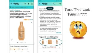
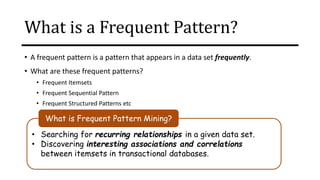
![Market Basket Analysis
• Buying patterns which reflect items frequently purchased or associated together
can be represented in rules form, known as association rules.
• e.g.
{𝑴𝒐𝒃𝒊𝒍𝒆} ⇒ 𝑺𝒄𝒓𝒆𝒆𝒏𝑮𝒖𝒂𝒓𝒅, 𝑩𝒂𝒄𝒌𝒄𝒐𝒗𝒆𝒓 [𝑠𝑢𝑝𝑝𝑜𝑟𝑡 = 5%, 𝑐𝑜𝑛𝑓𝑖𝑑𝑒𝑛𝑐𝑒 = 65%]
• Interestingness measures: 𝑺𝒖𝒑𝒑𝒐𝒓𝒕 and 𝑪𝒐𝒏𝒇𝒊𝒅𝒆𝒏𝒄𝒆
• Reflect the usefulness and certainty of discovered rules.
• Association rules are considered interesting if they satisfy both a minimum support
threshold and a minimum confidence threshold.
• Thresholds can be set by users or domain experts.](https://image.slidesharecdn.com/mdule5miningfrequentpatternsandassociationrules-220731073755-273a6dd8/85/Mining-Frequent-Patterns-And-Association-Rules-7-320.jpg)
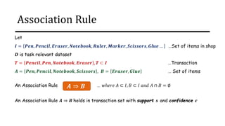


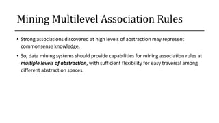
![Mining Multilevel Association Rules
• A serious side effect of mining multilevel association rules is its generation of many
redundant rules across multiple levels of abstraction due to the “ancestor”
relationships among items.
𝑏𝑢𝑦𝑠(𝑋, "Laptop computer") ⇒ 𝑏𝑢𝑦𝑠(𝑋, "HP Printer")
[𝑠𝑢𝑝𝑝𝑜𝑟𝑡 = 8%, 𝑐𝑜𝑛𝑓𝑖𝑑𝑒𝑛𝑐𝑒 = 70%]
𝑏𝑢𝑦𝑠(𝑋, "IBM Laptop computer") ⇒ 𝑏𝑢𝑦𝑠(𝑋, "HP Printer")
[𝑠𝑢𝑝𝑝𝑜𝑟𝑡 = 2%, 𝑐𝑜𝑛𝑓𝑖𝑑𝑒𝑛𝑐𝑒 = 72%]
• Does the later rule really provide any novel information??
• A rule 𝑅1 is an ancestor of a rule 𝑅2, if 𝑅1 can be obtained by replacing the items in
𝑅2 by their ancestors in a concept hierarchy.](https://image.slidesharecdn.com/mdule5miningfrequentpatternsandassociationrules-220731073755-273a6dd8/85/Mining-Frequent-Patterns-And-Association-Rules-81-320.jpg)

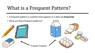
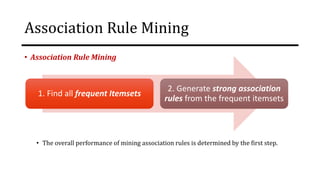
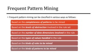
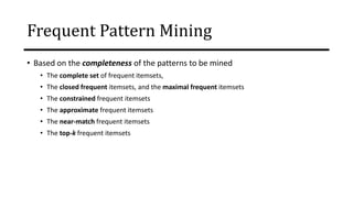
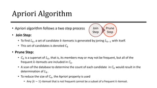
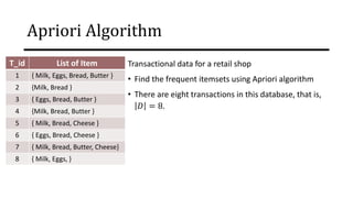
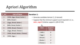
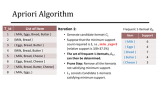
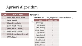
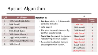
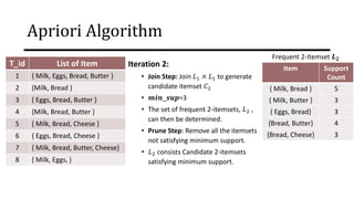
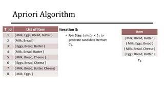
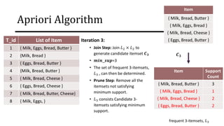
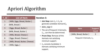
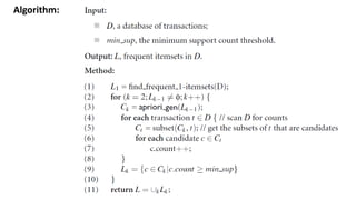
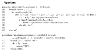
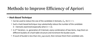
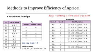
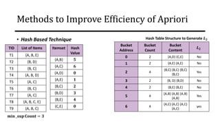
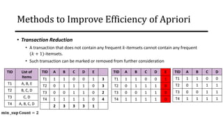
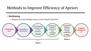
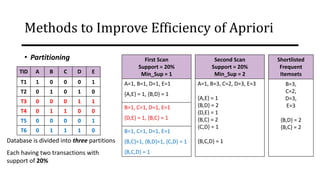
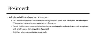
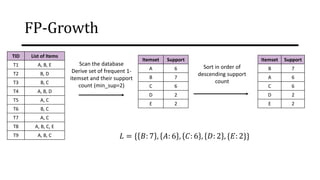
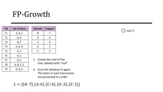
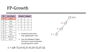
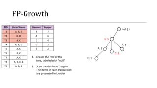
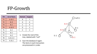
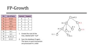
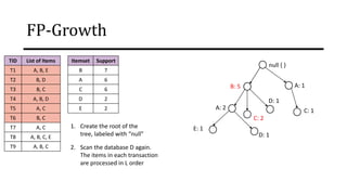
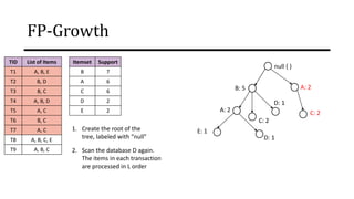
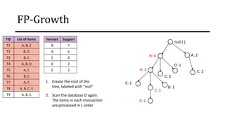
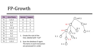
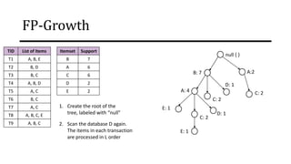
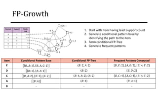
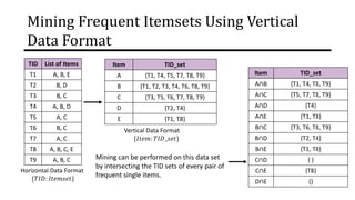
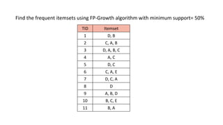
The document discusses frequent pattern mining and association rule mining. It defines key concepts like frequent itemsets, association rules, support and confidence. It explains the Apriori algorithm for mining frequent itemsets in multiple steps. The algorithm uses a level-wise search approach and the Apriori property to reduce the search space. It generates candidate itemsets in the join step and determines frequent itemsets by pruning infrequent candidates in the prune step. An example applying the Apriori algorithm to a retail transaction database is also provided to illustrate the working of the algorithm.