Downloaded 16 times


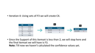


![Rules
• Confidence –
• A confidence of 60% means that 60% of the customers, who purchased milk and bread also bought butter.
• Confidence(A->B)=Support_count(A∪B)/Support_count(A)
• So here, by taking an example of any frequent itemset, we will show the rule generation.
• Itemset {I1, I2, I3} //from L3
• SO rules can be
• [I1^I2]=>[I3] //confidence = sup(I1^I2^I3)/sup(I1^I2) = 2/4*100=50%
• [I1^I3]=>[I2] //confidence = sup(I1^I2^I3)/sup(I1^I3) = 2/4*100=50%
• [I2^I3]=>[I1] //confidence = sup(I1^I2^I3)/sup(I2^I3) = 2/4*100=50%
• [I1]=>[I2^I3] //confidence = sup(I1^I2^I3)/sup(I1) = 2/6*100=33%
• [I2]=>[I1^I3] //confidence = sup(I1^I2^I3)/sup(I2) = 2/7*100=28%
• [I3]=>[I1^I2] //confidence = sup(I1^I2^I3)/sup(I3) = 2/6*100=33%
• So if minimum confidence is 50%, then first 3 rules can be considered as strong association rules.](https://image.slidesharecdn.com/associationrulemining-200330152358/85/Association-rule-mining-26-320.jpg)


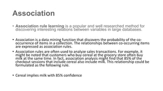
The document discusses association rule mining and the Apriori and FP-Growth algorithms. It provides the following information: - Association rule mining discovers interesting relationships between variables in large databases. It expresses relationships between frequently co-occurring items as association rules. - The Apriori algorithm uses frequent itemsets to generate association rules. It employs an iterative approach and pruning to reduce candidate sets. - FP-Growth improves upon Apriori by compressing transaction data into a frequent-pattern tree structure and scanning the database twice instead of multiple times. This improves mining efficiency over Apriori.