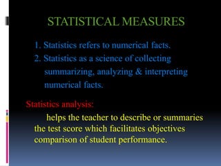
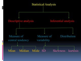
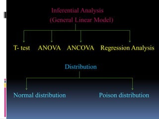
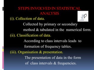
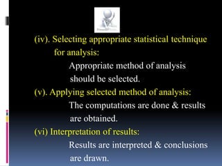
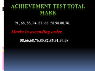
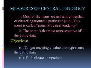
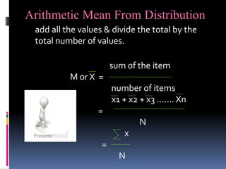
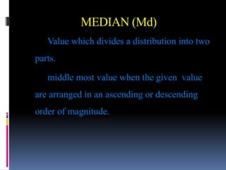
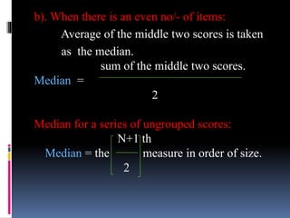
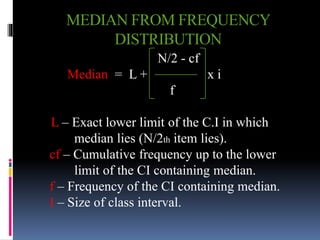
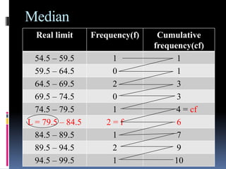
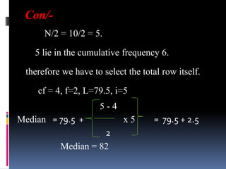
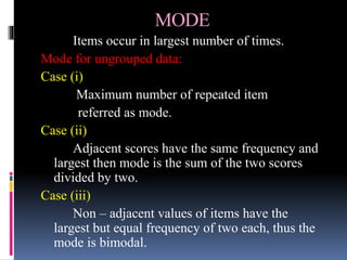
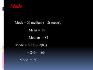
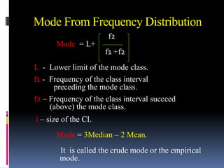
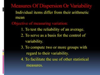
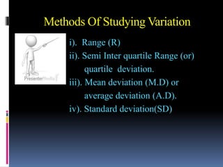
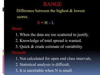
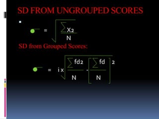
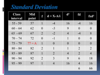
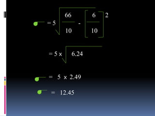
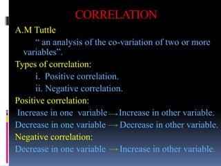
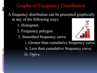
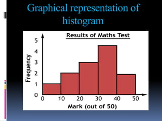
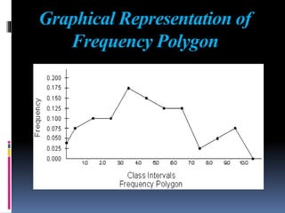
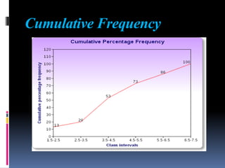
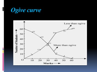
V. SURESH KUMAR
Assistant Professor In Mathematics
Rajalakshmi College Of Education
Thoothukudi
STATISTICAL MEASURES
1. Statistics refers to numerical facts.
2. Statistics as a science of collecting
summarizing, analyzing & interpreting
numerical facts.
Statistics analysis:
helps the teacher to describe or summaries
the test score which facilitates objectives
comparison of student performance.
Statistical Analysis
Descriptive analysis Inferential analysis
Measure of Measure of Distribution
central tendency variability
Mean Median Mode SD Skewness kurtosis
Inferential Analysis
(General Linear Model)
T- test ANOVA ANCOVA Regression Analysis
Distribution
Normal distribution Poison distribution
STEPS INVOLVED IN STATISTICAL
ANALYSIS
(i). Collection of data.
Collected by primary or secondary
method & tabulated in the numerical form.
(ii). Classification of data.
According to class intervals leads to
formation of frequency tables.
(iii). Organisation & presentation.
The presentation of data in the form
of class intervals & frequencies.
(iv). Selecting appropriate statistical technique
for analysis:
Appropriate method of analysis
should be selected.
(v). Applying selected method of analysis:
The computations are done & results
are obtained.
(vi) Interpretation of results:
Results are interpreted & conclusions
are drawn.
91, 68, 85, 94, 82, 66, 58,98,80,76.
Marks in ascending order.
58,66,68,76,80,82,85,91,94,98
Class
interval
Real limit Tally Frequency
55 – 59 54.5 – 59.5 l 1
60 - 64 59.5 – 64.5 0 0
65 – 69 64.5 – 69.5 ll 2
70 – 74 69.5 – 74.5 0 0
75 – 79 74.5 – 79.5 l 1
80 – 84 79.5 – 84.5 ll 2
85 – 89 84.5 – 89.5 l 1
90 – 94 89.5 – 94.5 ll 2
95 – 99 94.5 – 99.5 l 1
MEASURES OF CENTRALTENDENCY
1. Most of the items are gathering together
or clustering around a particular point. This
point is called “point of central tendency”.
2. The point is the most representative of
the entire data.
Objectives:
(i). To get one single value that represents
the entire data.
(ii). To facilitate comparison
Arithmetic Mean From Distribution
add all the values & divide the total by the
total number of values.
sum of the item
M or X =
number of items
x1 + x2 + x3 ……. Xn
=
N
x
=
N
58,66,68,76,80,82,85,91,94,98
sum of the items
X =
number of items
= 58 +66+68+76+80+82+85+91+94+98
10
= 704
10
= 70.4
Arithmetic Mean From Frequency
Distribution
1. Arithmetic mean by long method.
2. Arithmetic mean by short method.
Arithmetic Mean by Long Method
fx
X =
N
By short method (Assumed Mean Method):
fd
X = A.M + x i
N
X - AM
d(deviation) =
i
A.M – Assumed Mean
fd
X =A + × i
N
Class
interval
Mid point
(X)
f d = X – A / i fd
55 – 59 57 1 -4 -4
60 – 64 62 0 -3 0
65 - 69 67 2 -2 -4
70 – 74 72 0 -1 0
75 – 79 77 = A 1 0 0
80 – 84 82 2 1 2
85 – 89 87 1 2 2
90 – 94 92 2 3 6
95 – 99 97 1 4 4
6
Con/-
77- 57 - 20
d = = = - 4.
5 5
6
X = 77 + x 10
5
X = 89
MEDIAN (Md)
Value which divides a distribution into two
parts.
middle most value when the given value
are arranged in an ascending or descending
order of magnitude.
b). When there is an even no/- of items:
Average of the middle two scores is taken
as the median.
sum of the middle two scores.
Median =
2
Median for a series of ungrouped scores:
N+1 th
Median = the measure in order of size.
2
MEDIAN FROM FREQUENCY
DISTRIBUTION
N/2 - cf
Median = L + x i
f
L – Exact lower limit of the C.I in which
median lies (N/2th item lies).
cf – Cumulative frequency up to the lower
limit of the CI containing median.
f – Frequency of the CI containing median.
I – Size of class interval.
Median
Real limit Frequency(f) Cumulative
frequency(cf)
54.5 – 59.5 1 1
59.5 – 64.5 0 1
64.5 – 69.5 2 3
69.5 – 74.5 0 3
74.5 – 79.5 1 4 = cf
L = 79.5 – 84.5 2 = f 6
84.5 – 89.5 1 7
89.5 – 94.5 2 9
94.5 – 99.5 1 10
Con/-
N/2 = 10/2 = 5.
5 lie in the cumulative frequency 6.
therefore we have to select the total row itself.
cf = 4, f=2, L=79.5, i=5
5 - 4
Median = 79.5 + x 5 = 79.5 + 2.5
2
Median = 82
MODE
Items occur in largest number of times.
Mode for ungrouped data:
Case (i)
Maximum number of repeated item
referred as mode.
Case (ii)
Adjacent scores have the same frequency and
largest then mode is the sum of the two scores
divided by two.
Case (iii)
Non – adjacent values of items have the
largest but equal frequency of two each, thus the
mode is bimodal.
Mode
Mode = 3( median ) – 2( mean).
Mean = 89
Median = 82
Mode = 3(82) – 2(83)
= 246 – 166.
Mode = 80
Mode From Frequency Distribution
f2
Mode = L+
f1 +f2
L - Lower limit of the mode class.
f1 - Frequency of the class interval
preceding the mode class.
f2 – Frequency of the class interval succeed
(above) the mode class.
i – size of the CI.
Mode = 3Median – 2 Mean.
It is called the crude mode or the empirical
mode.
Measures Of Dispersion Or Variability
Individual items differ from their arithmetic
mean
Objective of measuring variation:
1. To test the reliability of an average.
2. To serve as a basis for the control of
variability.
3. To compute two or more groups with
regard to their variability.
4. To facilitate the use of other statistical
measures.
Methods Of Studying Variation
i). Range (R)
ii). Semi Inter quartile Range (or)
quartile deviation.
iii). Mean deviation (M.D) or
average deviation (A.D).
iv). Standard deviation(SD)
RANGE
Difference between the highest & lowest
scores.
R = H – L
Merit:
1. When the data are too scattered to justify.
2. Knowledge of total spread is wanted.
3. Quick & crude estimate of variability.
Demerit:
1. Not calculated for open end class intervals.
2. Statistical analysis is difficult.
3. It is unreliable when N is small.
Range
Range = Highest value – Lowest value.
= 98 – 58
= 40
The Semi – Inter – Quartile Range or Q
1. Extreme items is discarded, the limited
range is more instructive.
2. For this purpose, inter – quartile range –
developed.
lowest lower upper upper
quartile middle middle most
quartile quartile quartile
Q1 Q2 Q3
3. Half of the inter – quartile range or semi
– inter – quartile range is called the quartile
deviation (Q)
Q3 - Q1
Q =
2
N/4 – c.f
Q1 = L1 + x i
f
3N/4 – c.f
Q3 = L3 + x i
f
Quartile Deviation
Real limit Frequency Cumulative
frequency
54.5 – 59.5 1 1
59.5 – 64.5 0 1
64.5 – 69.5 2 3 = cf
L= 69.5 – 74.5 0 = f 3 Q1
74.5 – 79.5 1 4
79.5 – 84.5 2 6
84.5 – 89.5 1 7 = cf
L= 89.5 – 94.5 2 = f 9 Q3
94.5 – 99.5 1 10
Q3
3N/4 = 3(10)/4 = 7.5
L = 89.5, f= 2, cf = 7
7.5 - 7
Q3 = 89.5 + x 5
4
= 89.5 + 1.25
Q3 = 90.75
Q1
N/4 = 10/4 = 2.5
L = 69.5, f = 0, cf = 3
2.5 – 3
Q1 = 69.5 + x 5
0
Q1 = 69.5 +0
Q1 = 69.5
Q3 – Q1
Q =
2
90.75 – 69.5
Q = = 10.625
2
Q = 10.625
Average Deviation (AD) or Mean
Deviation
Average distance between the mean & scores
in the distribution.
X
A.D =
N
X = X – M
= absolute value of
deviation.
N – total No/- of scores.
Standard Deviation (S.D) or Rho
1. Introduced by karl pearson in 1893.
2. Most reliable & stable index of variability.
3. Greek letter sigma “ ”.
4. A standard unit for measuring distances of
various score from their mean.
In verbal term:
1. SD is the square root of the arithmetic mean
of the squared deviations of measurement
from their mean.
2. It is also called Root – Mean Square
Deviation.
SD FROM UNGROUPED SCORES

= X2
N
SD from Grouped Scores:
fd2 fd 2
= i x -
N N
Standard Deviation
Class
interval
Mid
point
f d = X-A/i
d²
[
fd
fxd²
55 - 59 57 1 -4 16 -4 16
60 – 64 62 0 -3 9 0 0
65 - 69 67 2 -2 4 -4 8
70 – 74 72 0 -1 1 0 0
75 – 79 77 = A 1 0 0 0 0
80 – 84 82 2 1 1 2 2
85 – 89 87 1 2 4 2 4
90 – 94 92 2 3 9 6 18
95 – 99 97 1 4 16 4 16
6 66
66 6 2
= 5 -
10 10
= 5 x 6.24
= 5 x 2.49
= 12.45
CORRELATION
A.M Tuttle
“ an analysis of the co-variation of two or more
variables”.
Types of correlation:
i. Positive correlation.
ii. Negative correlation.
Positive correlation:
Increase in one variable Increase in other variable.
Decrease in one variable Decrease in other variable.
Negative correlation:
Decrease in one variable Increase in other variable.
Linear & Non – Linear Correlation
1. Variation in the values of two values of
two variables are in constant ratio.
2. Y = a + bx – relationship.
Coefficient of correlation (r):
1. To study the extent or degree of correlation
between two variable.
2. Represent by the letter r.
The range of r:
1. Correlation coefficient may assume values
from 0 to 1
2. Minus (-) & plus(+) sign indicate the
relationship +ve or –ve.
r In Terms of Verbal Description
value of r verbal description
± 0.00 to ± 0.20 Independent or
negligible relationship
±0.20 to ± 0.40 Low correlation present
±0.40 to ± 0.70 Substantial or marked
± 0.70 to ±1.00 High to very high
Computation of Correlation Coefficient
1. Spearman’s Rank – difference method .
2. Pearson’s product moment method.
Spearman’s Rank Difference correlation
coefficient ( (Rho)
6 D²
( = 1 -
N (N -1)
D – Difference in ranks.
Rank correlation
Mark 1 Rank 1 Mark 2 Rank 2 D = R1-R2 D²
58 10 70 8 2 4
68 8 90 1 7 49
66 9 71 7 2 4
76 7 89 2 5 25
85 4 53 9 5 25
82 5 76 5 0 0
80 6 49 10 4 16
98 1 88 3 2 4
94 2 73 6 4 16
91 3 86 4 1 1
144
Con/-
1 – (6 x144)
ρ =
10 (10 x10 -1)
1 - 864
ρ = = - 0.8717
990
Therefore ρ = - 0.87. his indicates a
strong negative relationship between the ranks
individuals obtained in the Math & English
exam.
Graphical Representation of Data
Graph:
1. Frequency distributions are converted into
visual models to facilitate understanding.
2. Data may be presented through diagrams &
graphs.
Graphs of Frequency Distribution
A frequency distribution can be presented graphically
in any of the following ways.
1. Histogram.
2. Frequency polygon.
3. Smoothed frequency curve.
i. Greater than cumulative frequency curve.
ii. Less than cumulative frequency curve.
iii. Ogive.
Graphical representation of
histogram
Graphical Representation of
Frequency Polygon
Cumulative Frequency
Ogive curve
test & measuement

test & measuement

  • 1.
    V. SURESH KUMAR AssistantProfessor In Mathematics Rajalakshmi College Of Education Thoothukudi
  • 2.
    STATISTICAL MEASURES 1. Statisticsrefers to numerical facts. 2. Statistics as a science of collecting summarizing, analyzing & interpreting numerical facts. Statistics analysis: helps the teacher to describe or summaries the test score which facilitates objectives comparison of student performance.
  • 3.
    Statistical Analysis Descriptive analysisInferential analysis Measure of Measure of Distribution central tendency variability Mean Median Mode SD Skewness kurtosis
  • 4.
    Inferential Analysis (General LinearModel) T- test ANOVA ANCOVA Regression Analysis Distribution Normal distribution Poison distribution
  • 5.
    STEPS INVOLVED INSTATISTICAL ANALYSIS (i). Collection of data. Collected by primary or secondary method & tabulated in the numerical form. (ii). Classification of data. According to class intervals leads to formation of frequency tables. (iii). Organisation & presentation. The presentation of data in the form of class intervals & frequencies.
  • 6.
    (iv). Selecting appropriatestatistical technique for analysis: Appropriate method of analysis should be selected. (v). Applying selected method of analysis: The computations are done & results are obtained. (vi) Interpretation of results: Results are interpreted & conclusions are drawn.
  • 7.
    91, 68, 85,94, 82, 66, 58,98,80,76. Marks in ascending order. 58,66,68,76,80,82,85,91,94,98
  • 8.
    Class interval Real limit TallyFrequency 55 – 59 54.5 – 59.5 l 1 60 - 64 59.5 – 64.5 0 0 65 – 69 64.5 – 69.5 ll 2 70 – 74 69.5 – 74.5 0 0 75 – 79 74.5 – 79.5 l 1 80 – 84 79.5 – 84.5 ll 2 85 – 89 84.5 – 89.5 l 1 90 – 94 89.5 – 94.5 ll 2 95 – 99 94.5 – 99.5 l 1
  • 9.
    MEASURES OF CENTRALTENDENCY 1.Most of the items are gathering together or clustering around a particular point. This point is called “point of central tendency”. 2. The point is the most representative of the entire data. Objectives: (i). To get one single value that represents the entire data. (ii). To facilitate comparison
  • 10.
    Arithmetic Mean FromDistribution add all the values & divide the total by the total number of values. sum of the item M or X = number of items x1 + x2 + x3 ……. Xn = N x = N
  • 11.
    58,66,68,76,80,82,85,91,94,98 sum of theitems X = number of items = 58 +66+68+76+80+82+85+91+94+98 10 = 704 10 = 70.4
  • 12.
    Arithmetic Mean FromFrequency Distribution 1. Arithmetic mean by long method. 2. Arithmetic mean by short method.
  • 13.
    Arithmetic Mean byLong Method fx X = N By short method (Assumed Mean Method): fd X = A.M + x i N X - AM d(deviation) = i A.M – Assumed Mean
  • 14.
    fd X =A +× i N Class interval Mid point (X) f d = X – A / i fd 55 – 59 57 1 -4 -4 60 – 64 62 0 -3 0 65 - 69 67 2 -2 -4 70 – 74 72 0 -1 0 75 – 79 77 = A 1 0 0 80 – 84 82 2 1 2 85 – 89 87 1 2 2 90 – 94 92 2 3 6 95 – 99 97 1 4 4 6
  • 15.
    Con/- 77- 57 -20 d = = = - 4. 5 5 6 X = 77 + x 10 5 X = 89
  • 16.
    MEDIAN (Md) Value whichdivides a distribution into two parts. middle most value when the given value are arranged in an ascending or descending order of magnitude.
  • 17.
    b). When thereis an even no/- of items: Average of the middle two scores is taken as the median. sum of the middle two scores. Median = 2 Median for a series of ungrouped scores: N+1 th Median = the measure in order of size. 2
  • 18.
    MEDIAN FROM FREQUENCY DISTRIBUTION N/2- cf Median = L + x i f L – Exact lower limit of the C.I in which median lies (N/2th item lies). cf – Cumulative frequency up to the lower limit of the CI containing median. f – Frequency of the CI containing median. I – Size of class interval.
  • 19.
    Median Real limit Frequency(f)Cumulative frequency(cf) 54.5 – 59.5 1 1 59.5 – 64.5 0 1 64.5 – 69.5 2 3 69.5 – 74.5 0 3 74.5 – 79.5 1 4 = cf L = 79.5 – 84.5 2 = f 6 84.5 – 89.5 1 7 89.5 – 94.5 2 9 94.5 – 99.5 1 10
  • 20.
    Con/- N/2 = 10/2= 5. 5 lie in the cumulative frequency 6. therefore we have to select the total row itself. cf = 4, f=2, L=79.5, i=5 5 - 4 Median = 79.5 + x 5 = 79.5 + 2.5 2 Median = 82
  • 21.
    MODE Items occur inlargest number of times. Mode for ungrouped data: Case (i) Maximum number of repeated item referred as mode. Case (ii) Adjacent scores have the same frequency and largest then mode is the sum of the two scores divided by two. Case (iii) Non – adjacent values of items have the largest but equal frequency of two each, thus the mode is bimodal.
  • 22.
    Mode Mode = 3(median ) – 2( mean). Mean = 89 Median = 82 Mode = 3(82) – 2(83) = 246 – 166. Mode = 80
  • 23.
    Mode From FrequencyDistribution f2 Mode = L+ f1 +f2 L - Lower limit of the mode class. f1 - Frequency of the class interval preceding the mode class. f2 – Frequency of the class interval succeed (above) the mode class. i – size of the CI. Mode = 3Median – 2 Mean. It is called the crude mode or the empirical mode.
  • 24.
    Measures Of DispersionOr Variability Individual items differ from their arithmetic mean Objective of measuring variation: 1. To test the reliability of an average. 2. To serve as a basis for the control of variability. 3. To compute two or more groups with regard to their variability. 4. To facilitate the use of other statistical measures.
  • 25.
    Methods Of StudyingVariation i). Range (R) ii). Semi Inter quartile Range (or) quartile deviation. iii). Mean deviation (M.D) or average deviation (A.D). iv). Standard deviation(SD)
  • 26.
    RANGE Difference between thehighest & lowest scores. R = H – L Merit: 1. When the data are too scattered to justify. 2. Knowledge of total spread is wanted. 3. Quick & crude estimate of variability. Demerit: 1. Not calculated for open end class intervals. 2. Statistical analysis is difficult. 3. It is unreliable when N is small.
  • 27.
    Range Range = Highestvalue – Lowest value. = 98 – 58 = 40
  • 28.
    The Semi –Inter – Quartile Range or Q 1. Extreme items is discarded, the limited range is more instructive. 2. For this purpose, inter – quartile range – developed. lowest lower upper upper quartile middle middle most quartile quartile quartile Q1 Q2 Q3
  • 29.
    3. Half ofthe inter – quartile range or semi – inter – quartile range is called the quartile deviation (Q) Q3 - Q1 Q = 2 N/4 – c.f Q1 = L1 + x i f 3N/4 – c.f Q3 = L3 + x i f
  • 30.
    Quartile Deviation Real limitFrequency Cumulative frequency 54.5 – 59.5 1 1 59.5 – 64.5 0 1 64.5 – 69.5 2 3 = cf L= 69.5 – 74.5 0 = f 3 Q1 74.5 – 79.5 1 4 79.5 – 84.5 2 6 84.5 – 89.5 1 7 = cf L= 89.5 – 94.5 2 = f 9 Q3 94.5 – 99.5 1 10
  • 31.
    Q3 3N/4 = 3(10)/4= 7.5 L = 89.5, f= 2, cf = 7 7.5 - 7 Q3 = 89.5 + x 5 4 = 89.5 + 1.25 Q3 = 90.75 Q1 N/4 = 10/4 = 2.5 L = 69.5, f = 0, cf = 3
  • 32.
    2.5 – 3 Q1= 69.5 + x 5 0 Q1 = 69.5 +0 Q1 = 69.5 Q3 – Q1 Q = 2 90.75 – 69.5 Q = = 10.625 2 Q = 10.625
  • 33.
    Average Deviation (AD)or Mean Deviation Average distance between the mean & scores in the distribution. X A.D = N X = X – M = absolute value of deviation. N – total No/- of scores.
  • 34.
    Standard Deviation (S.D)or Rho 1. Introduced by karl pearson in 1893. 2. Most reliable & stable index of variability. 3. Greek letter sigma “ ”. 4. A standard unit for measuring distances of various score from their mean. In verbal term: 1. SD is the square root of the arithmetic mean of the squared deviations of measurement from their mean. 2. It is also called Root – Mean Square Deviation.
  • 35.
    SD FROM UNGROUPEDSCORES  = X2 N SD from Grouped Scores: fd2 fd 2 = i x - N N
  • 36.
    Standard Deviation Class interval Mid point f d= X-A/i d² [ fd fxd² 55 - 59 57 1 -4 16 -4 16 60 – 64 62 0 -3 9 0 0 65 - 69 67 2 -2 4 -4 8 70 – 74 72 0 -1 1 0 0 75 – 79 77 = A 1 0 0 0 0 80 – 84 82 2 1 1 2 2 85 – 89 87 1 2 4 2 4 90 – 94 92 2 3 9 6 18 95 – 99 97 1 4 16 4 16 6 66
  • 37.
    66 6 2 =5 - 10 10 = 5 x 6.24 = 5 x 2.49 = 12.45
  • 38.
    CORRELATION A.M Tuttle “ ananalysis of the co-variation of two or more variables”. Types of correlation: i. Positive correlation. ii. Negative correlation. Positive correlation: Increase in one variable Increase in other variable. Decrease in one variable Decrease in other variable. Negative correlation: Decrease in one variable Increase in other variable.
  • 39.
    Linear & Non– Linear Correlation 1. Variation in the values of two values of two variables are in constant ratio. 2. Y = a + bx – relationship. Coefficient of correlation (r): 1. To study the extent or degree of correlation between two variable. 2. Represent by the letter r. The range of r: 1. Correlation coefficient may assume values from 0 to 1 2. Minus (-) & plus(+) sign indicate the relationship +ve or –ve.
  • 40.
    r In Termsof Verbal Description value of r verbal description ± 0.00 to ± 0.20 Independent or negligible relationship ±0.20 to ± 0.40 Low correlation present ±0.40 to ± 0.70 Substantial or marked ± 0.70 to ±1.00 High to very high
  • 41.
    Computation of CorrelationCoefficient 1. Spearman’s Rank – difference method . 2. Pearson’s product moment method. Spearman’s Rank Difference correlation coefficient ( (Rho) 6 D² ( = 1 - N (N -1) D – Difference in ranks.
  • 42.
    Rank correlation Mark 1Rank 1 Mark 2 Rank 2 D = R1-R2 D² 58 10 70 8 2 4 68 8 90 1 7 49 66 9 71 7 2 4 76 7 89 2 5 25 85 4 53 9 5 25 82 5 76 5 0 0 80 6 49 10 4 16 98 1 88 3 2 4 94 2 73 6 4 16 91 3 86 4 1 1 144
  • 43.
    Con/- 1 – (6x144) ρ = 10 (10 x10 -1) 1 - 864 ρ = = - 0.8717 990 Therefore ρ = - 0.87. his indicates a strong negative relationship between the ranks individuals obtained in the Math & English exam.
  • 44.
    Graphical Representation ofData Graph: 1. Frequency distributions are converted into visual models to facilitate understanding. 2. Data may be presented through diagrams & graphs.
  • 45.
    Graphs of FrequencyDistribution A frequency distribution can be presented graphically in any of the following ways. 1. Histogram. 2. Frequency polygon. 3. Smoothed frequency curve. i. Greater than cumulative frequency curve. ii. Less than cumulative frequency curve. iii. Ogive.
  • 46.
  • 47.
  • 48.
  • 49.