Download to read offline
![Check data column wise
> data[,1]
> data[,2]
> data[,3]
> data[,4]
Find out mean
> mean(data[,1])
> mean(data[,2])
> mean(data[,3])
> mean(data[,4])](https://image.slidesharecdn.com/lecture9ba9rsoftware-190216050542/85/Lecture-9-ba-9-r-software-5-320.jpg)
![Calculation of MEDIAN
>median(data[,1])
>median(data[,2])
> median(data[,3])
> median(data[,4])](https://image.slidesharecdn.com/lecture9ba9rsoftware-190216050542/85/Lecture-9-ba-9-r-software-6-320.jpg)
![Calculation of SD
>sd(data[,1])
>sd(data[,2])
> sd(data[,3])
> sd(data[,4])](https://image.slidesharecdn.com/lecture9ba9rsoftware-190216050542/85/Lecture-9-ba-9-r-software-7-320.jpg)
![> gender<-c(1,2,1,1,2,1,2,1,2,1,2)
> gender
[1] 1 2 1 1 2 1 2 1 2 1 2
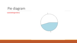
> table(gender)
gender
1 2
6 5
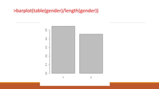
> table(gender)/length(gender)
gender
1 2
0.5454545 0.4545455](https://image.slidesharecdn.com/lecture9ba9rsoftware-190216050542/85/Lecture-9-ba-9-r-software-9-320.jpg)
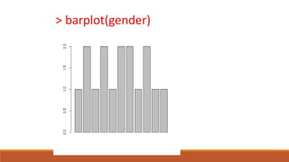
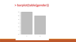
![Graphics and Plots
> gender<-c(1,2,1,2,1,2,2,1,2,1,1)
> gender
[1] 1 2 1 2 1 2 2 1 2 1 1
> table(gender)
gender
1 2
6 5
> barplot(table(gender))](https://image.slidesharecdn.com/lecture9ba9rsoftware-190216050542/85/Lecture-9-ba-9-r-software-10-320.jpg)
![Correlation
> cor(c(100,200,300,400),c(100,200,300,400))
[1] 1](https://image.slidesharecdn.com/lecture9ba9rsoftware-190216050542/85/Lecture-9-ba-9-r-software-16-320.jpg)
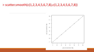
![Graph
> cor(c(1,2,3,4,5,6,7,8),c(1,2,3,4,5,6,7,8))
[1] 1
> plot(c(1,2,3,4,5,6,7,8),c(1,2,3,4,5,6,7,8))](https://image.slidesharecdn.com/lecture9ba9rsoftware-190216050542/85/Lecture-9-ba-9-r-software-17-320.jpg)

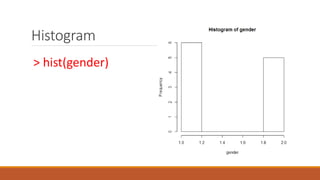
This document discusses importing data from CSV files into R and performing calculations and analysis on the data. It covers changing the working directory in R, importing CSV data and assigning column comments, and calculating summary statistics like the mean, median, and standard deviation of columns of data. It also demonstrates creating bar plots, pie charts, histograms and calculating the correlation between variables and fitting a linear regression model.