Downloaded 45 times
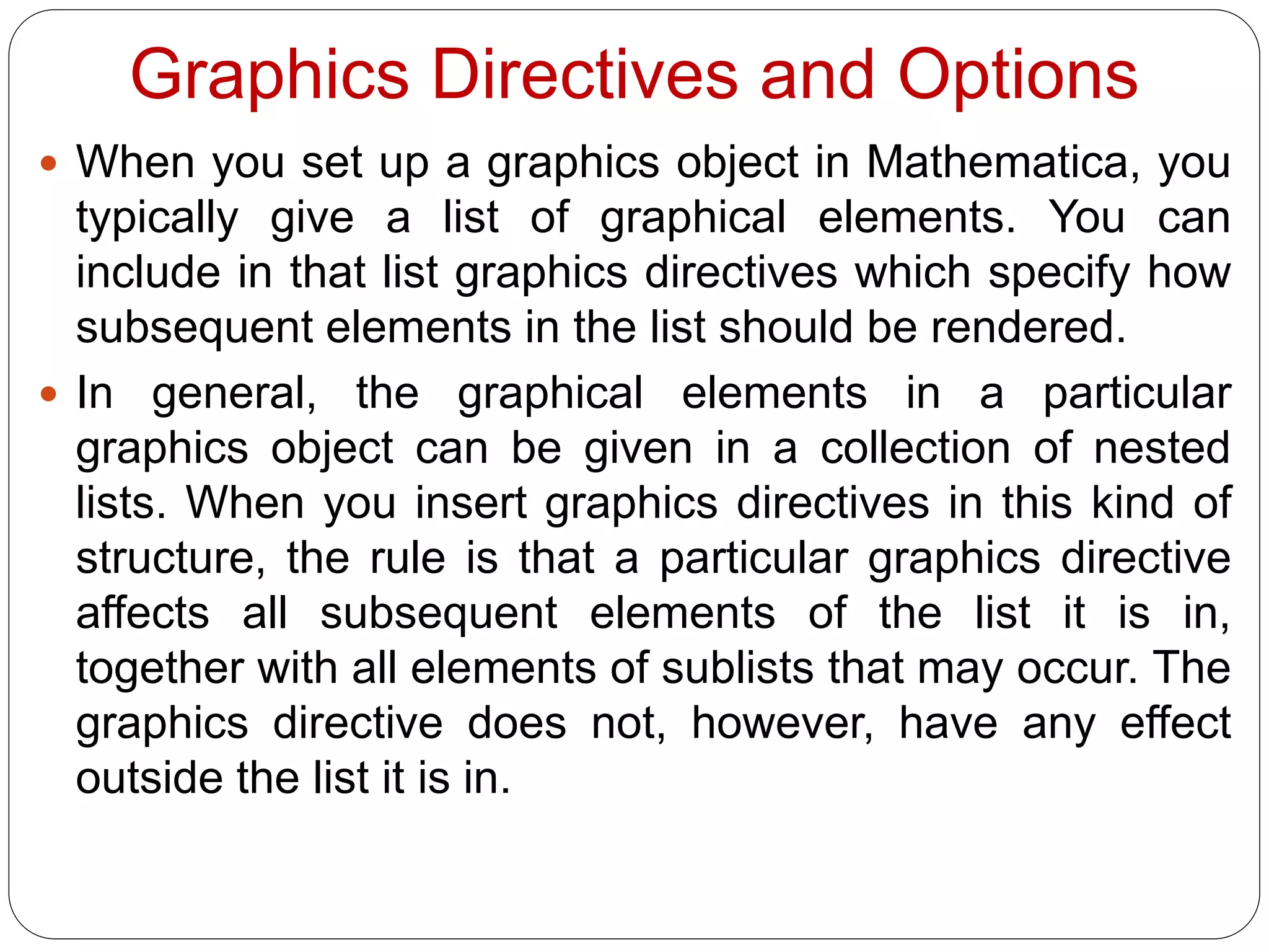
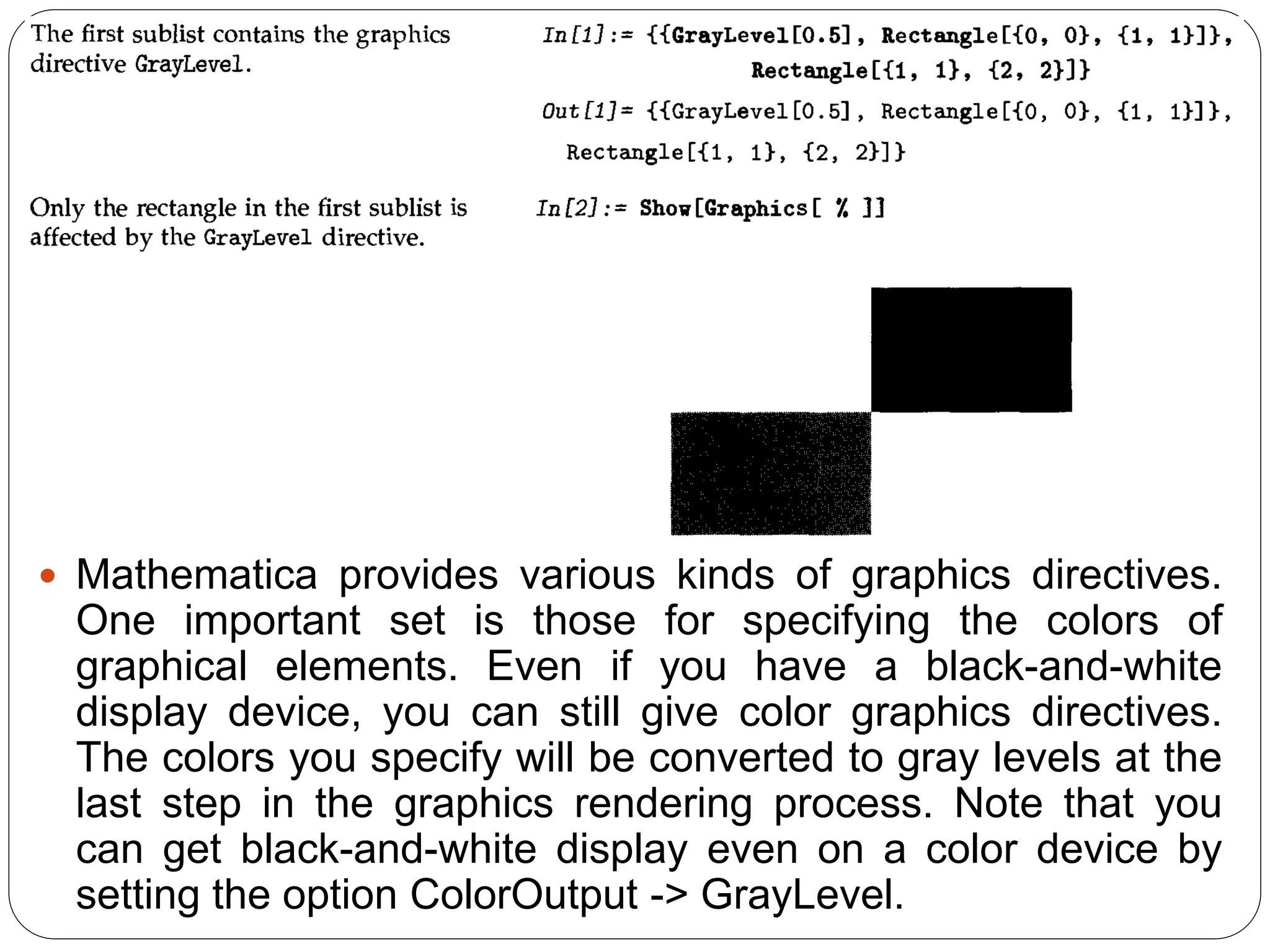
![To get smooth curves, Mathematica has to evaluate functions you plot at a large number of points. As a result, it is important that you set things up so that each function evaluation is as quick as possible.
When you ask Mathematica to plot an object, say f, as a function of x, there are two possible approaches it can take. One approach is first to try and evaluate f, presumably getting a symbolic expression in terms of x, and then subsequently evaluate this expression numerically for the specific values of x needed in the plot. The second approach is first to work out what values of x are needed, and only subsequently to evaluate f with those values of x.
If you type Plot [f, {x, xmin, xmax}] it is the second of these approaches that is used. This has the advantage that Mathematica only tries to evaluate f for specific numerical values of x; it does not matter whether sensible values are defined for f when x is symbolic.
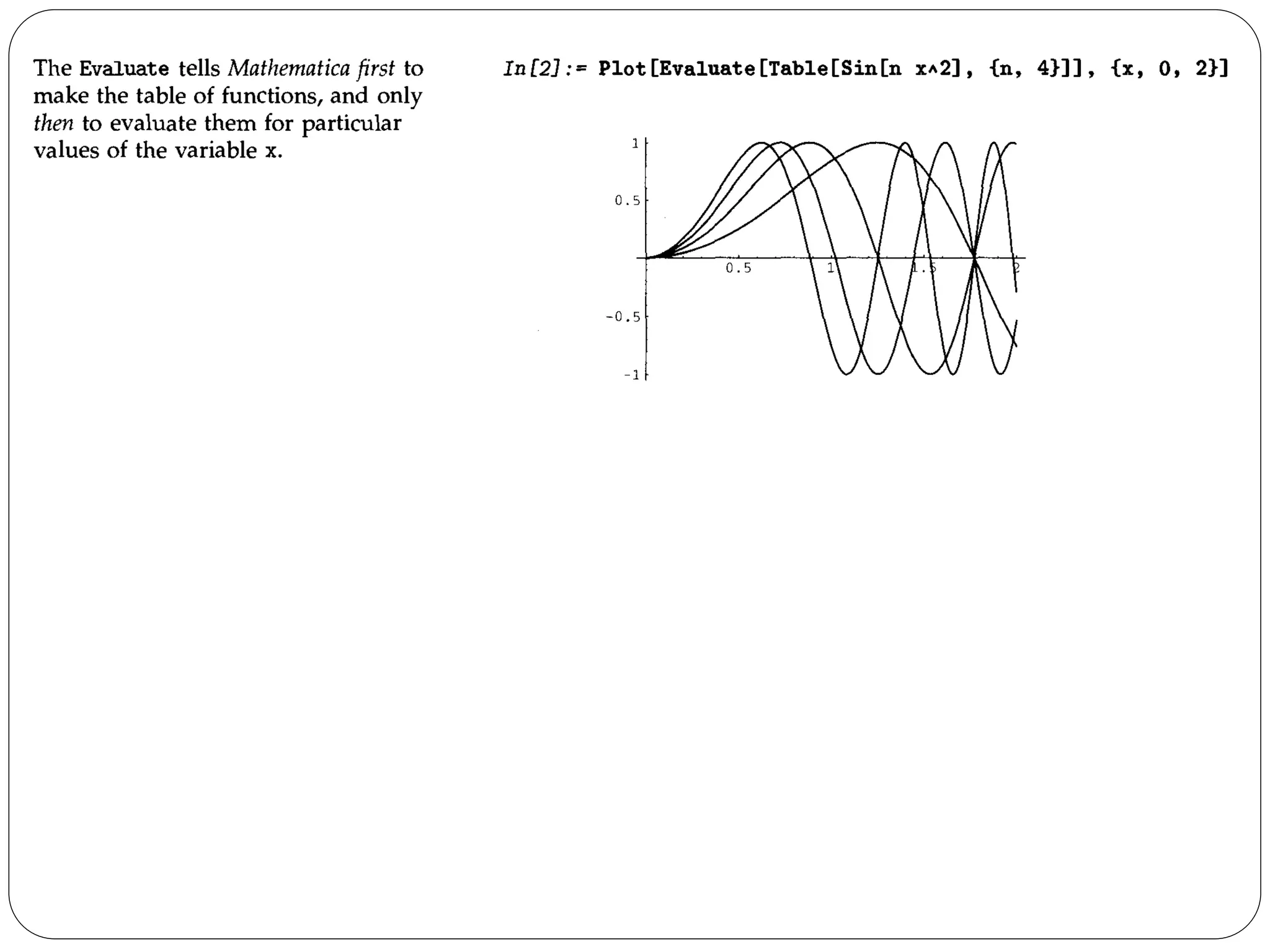
There are, however, some cases in which it is much better to have Mathematica evaluate f before it starts to make the plot. A typical case is when f is actually a command that generates a table of functions. You want to have Mathematica first produce the table, and then evaluate the functions, rather than trying to produce the table afresh for each value of x. You can do this by typing Plot [Evaluate [f] , {x, xmin, xmax}].](https://image.slidesharecdn.com/me443-4plottingcurves-141102125453-conversion-gate02/75/Me-443-4-plotting-curves-Erdi-Karacal-Mechanical-Engineer-University-of-Gaziantep-22-2048.jpg)
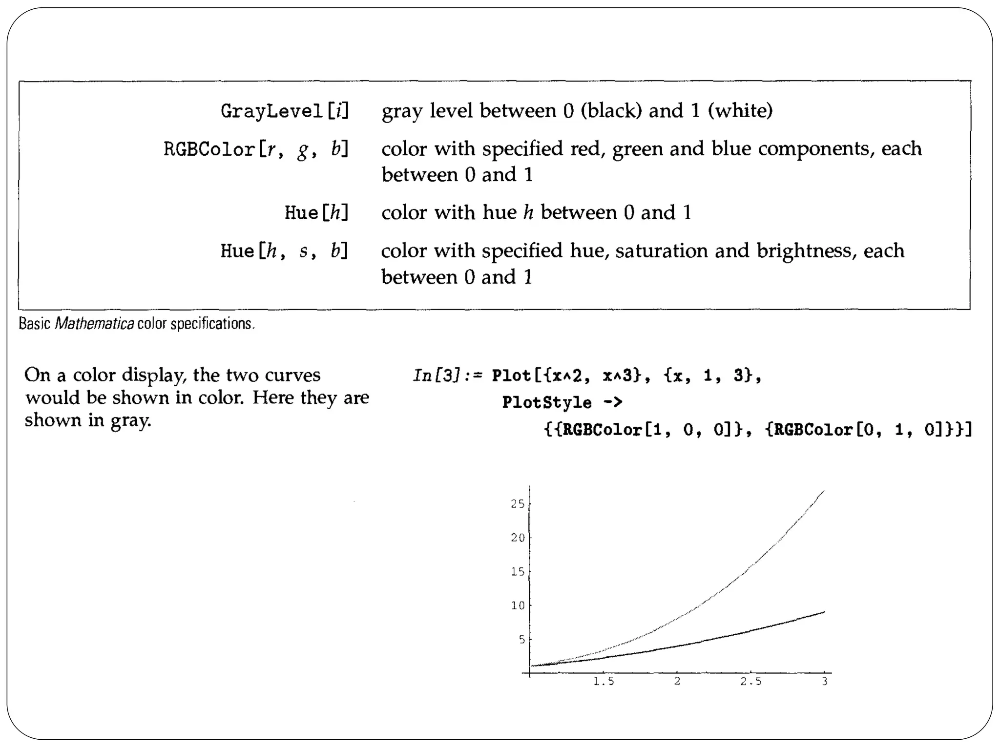
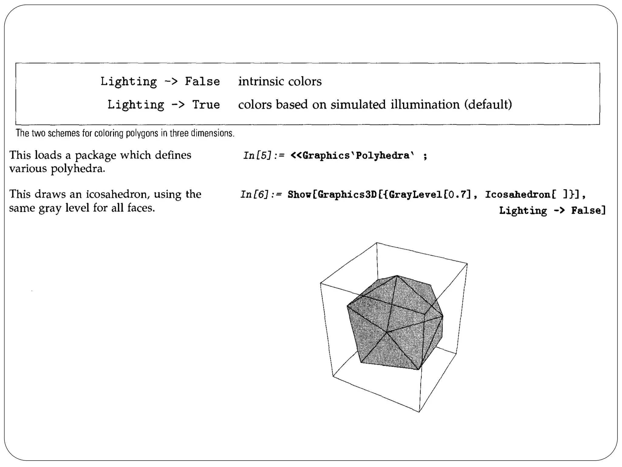
![The function Hue[h] provides a convenient way to specify a range of colors using just one parameter. As ft varies from 0 to 1, Hue[h] runs through red, yellow, green, cyan, blue, magenta, and back to red again. Hue [h, s, b] allows you to specify not only the "hue", but also the "saturation" and "brightness" of a color. Taking the saturation to be equal to one gives the deepest colors; decreasing the saturation towards zero leads to progressively more "washed out" colors.
For most purposes, you will be able to specify the colors you need simply by giving appropriate RGBColor or Hue directives.
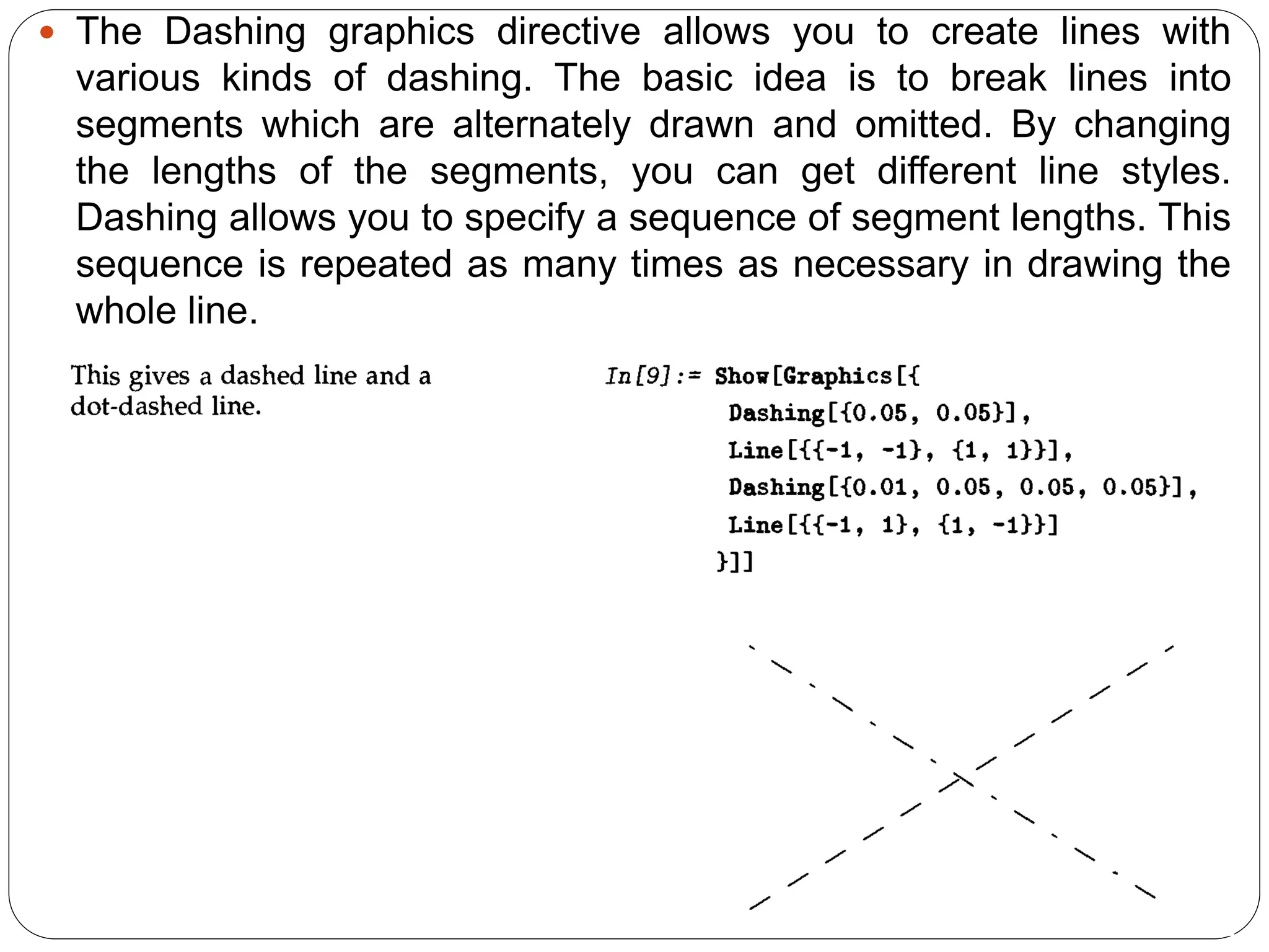
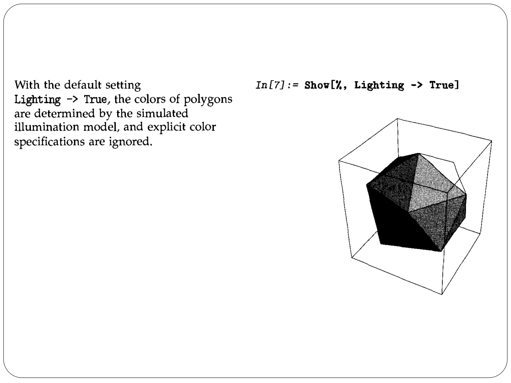
When you give a graphics directive such as RGBColor, it affects all subsequent graphical elements that appear in a particular list. Mathematica also supports various graphics directives which affect only specific types of graphical elements.](https://image.slidesharecdn.com/me443-4plottingcurves-141102125453-conversion-gate02/75/Me-443-4-plotting-curves-Erdi-Karacal-Mechanical-Engineer-University-of-Gaziantep-38-2048.jpg)
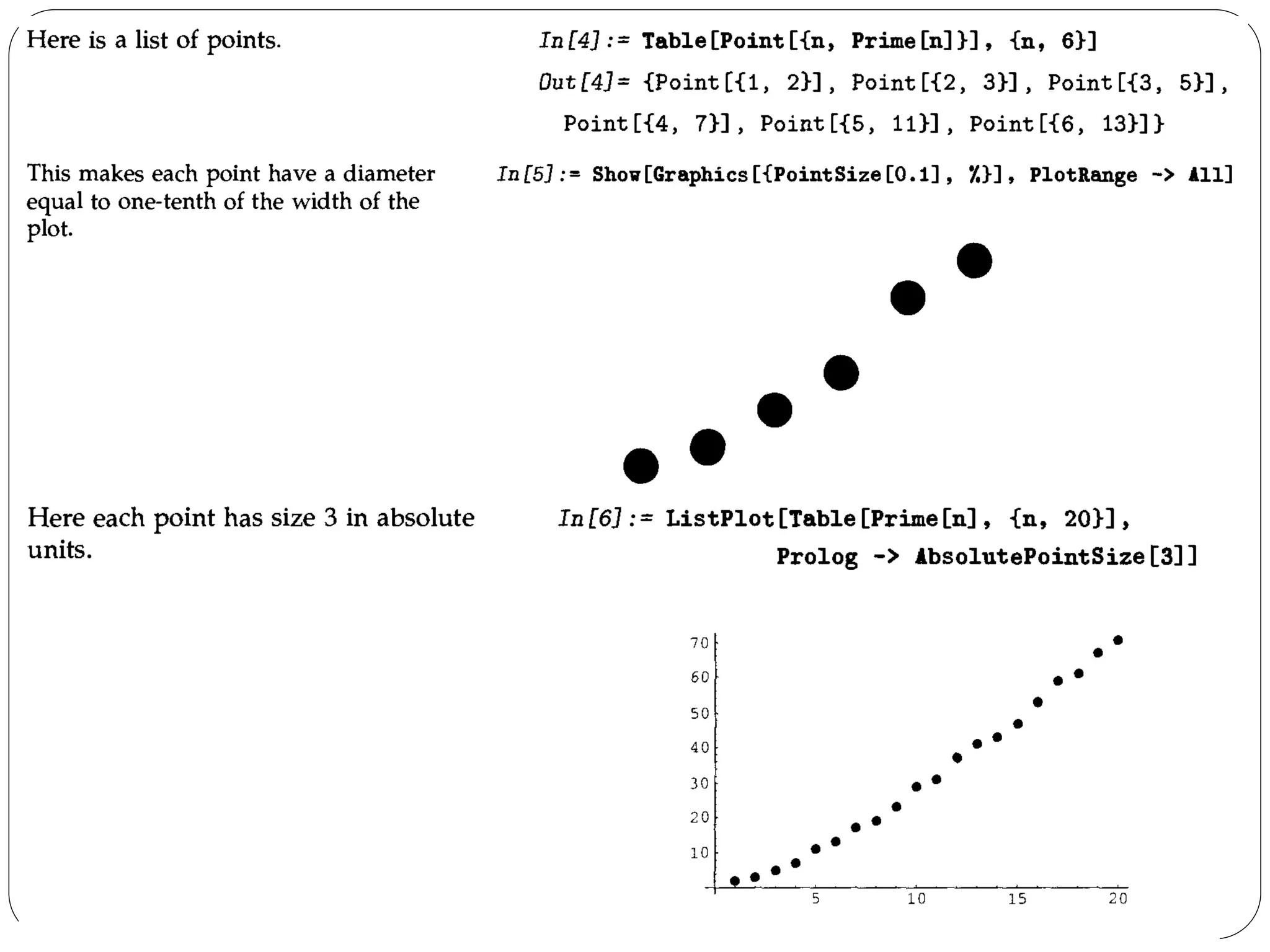
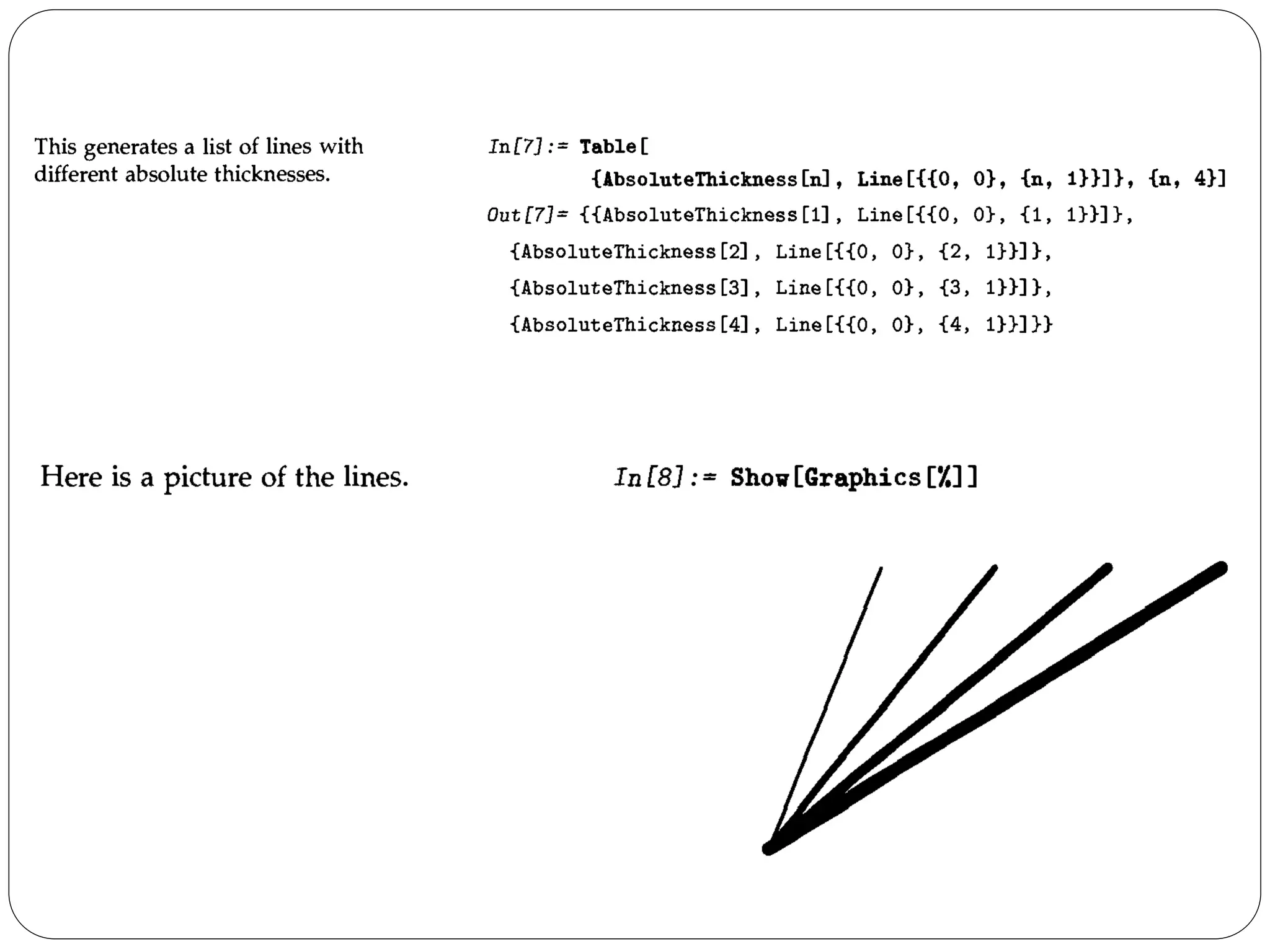
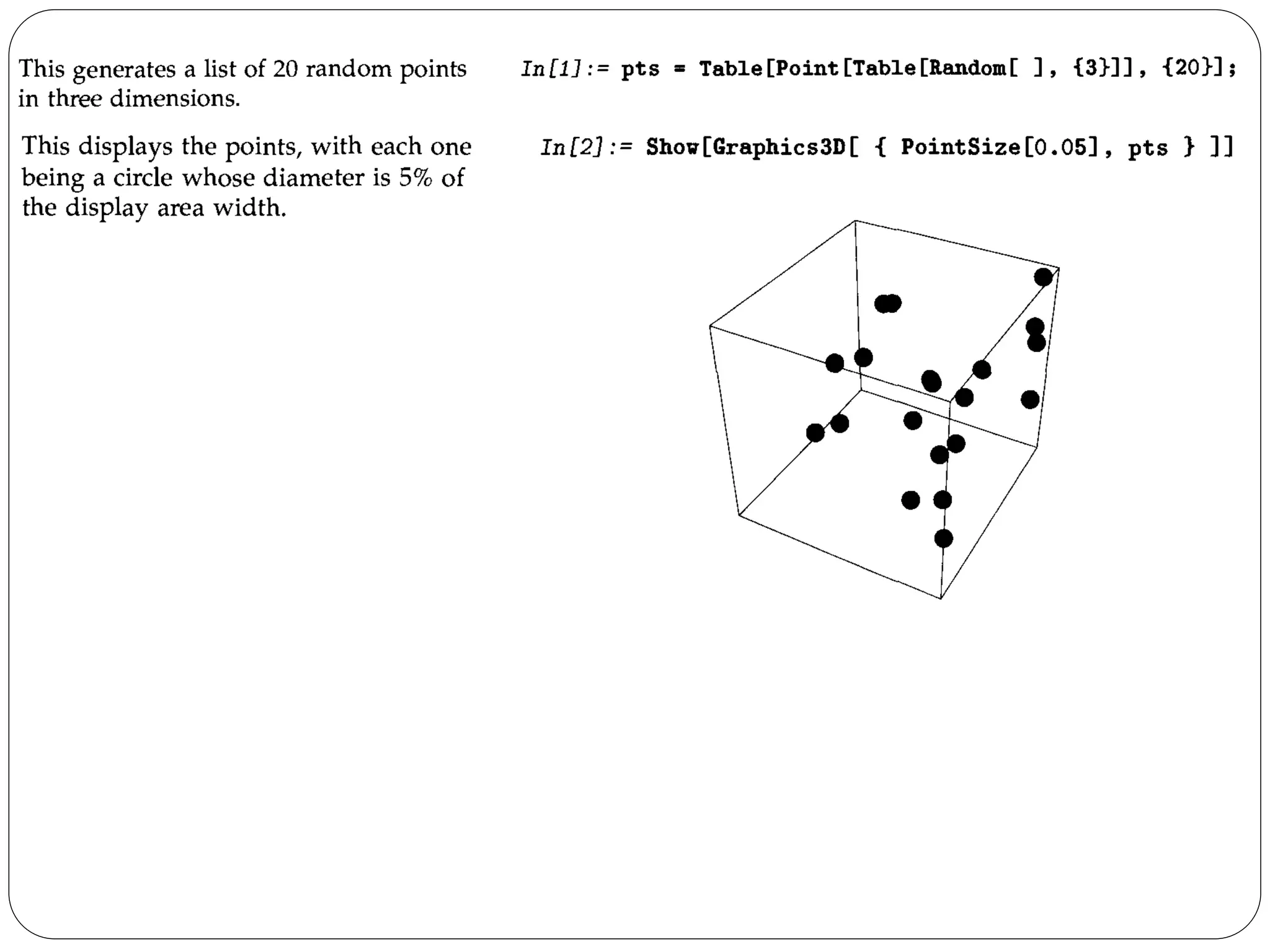
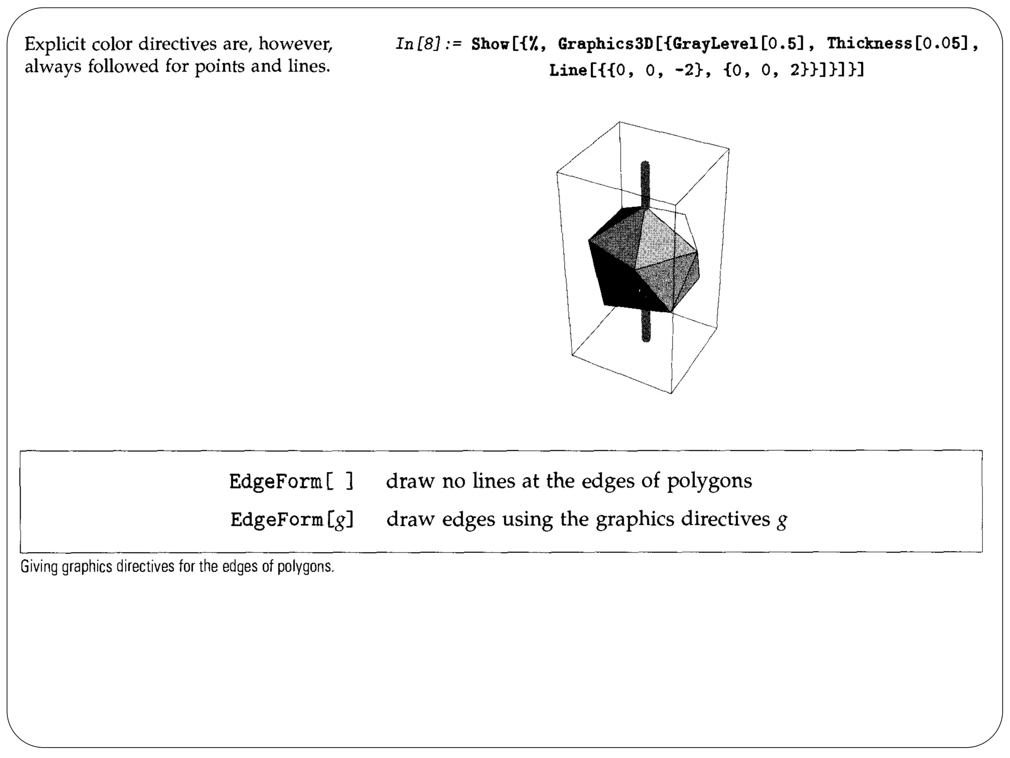
![The graphics directive PointSize[d] specifies that all Point elements which appear in a graphics object should be drawn as circles with a diameter d. In PointSize, the diameter d is measured as a fraction of the width of your whole plot.
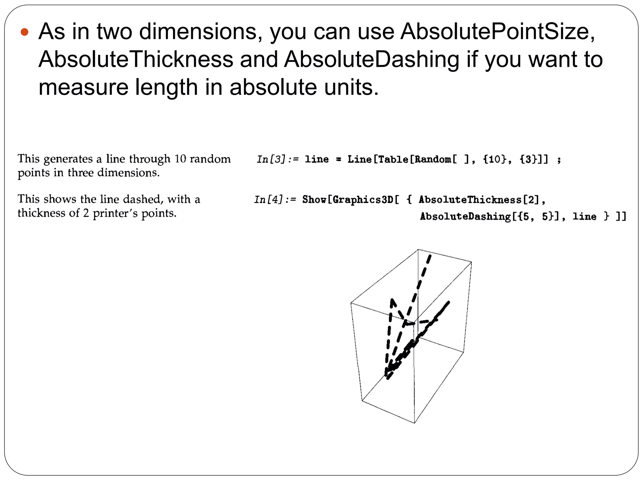
Mathematica also provides the graphics directive AbsolutePointSize[d], which allows you to specify the "absolute" diameter of points, measured in fixed units. The units are approximately printer's points, equal to 1/72 of an inch.](https://image.slidesharecdn.com/me443-4plottingcurves-141102125453-conversion-gate02/75/Me-443-4-plotting-curves-Erdi-Karacal-Mechanical-Engineer-University-of-Gaziantep-39-2048.jpg)

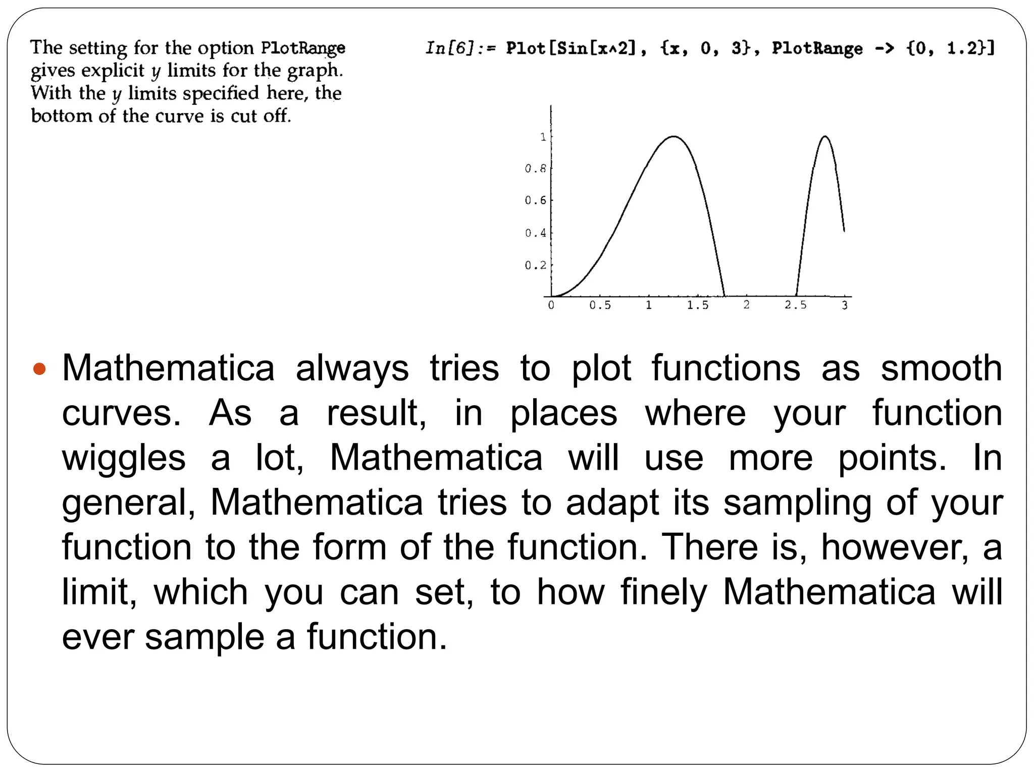
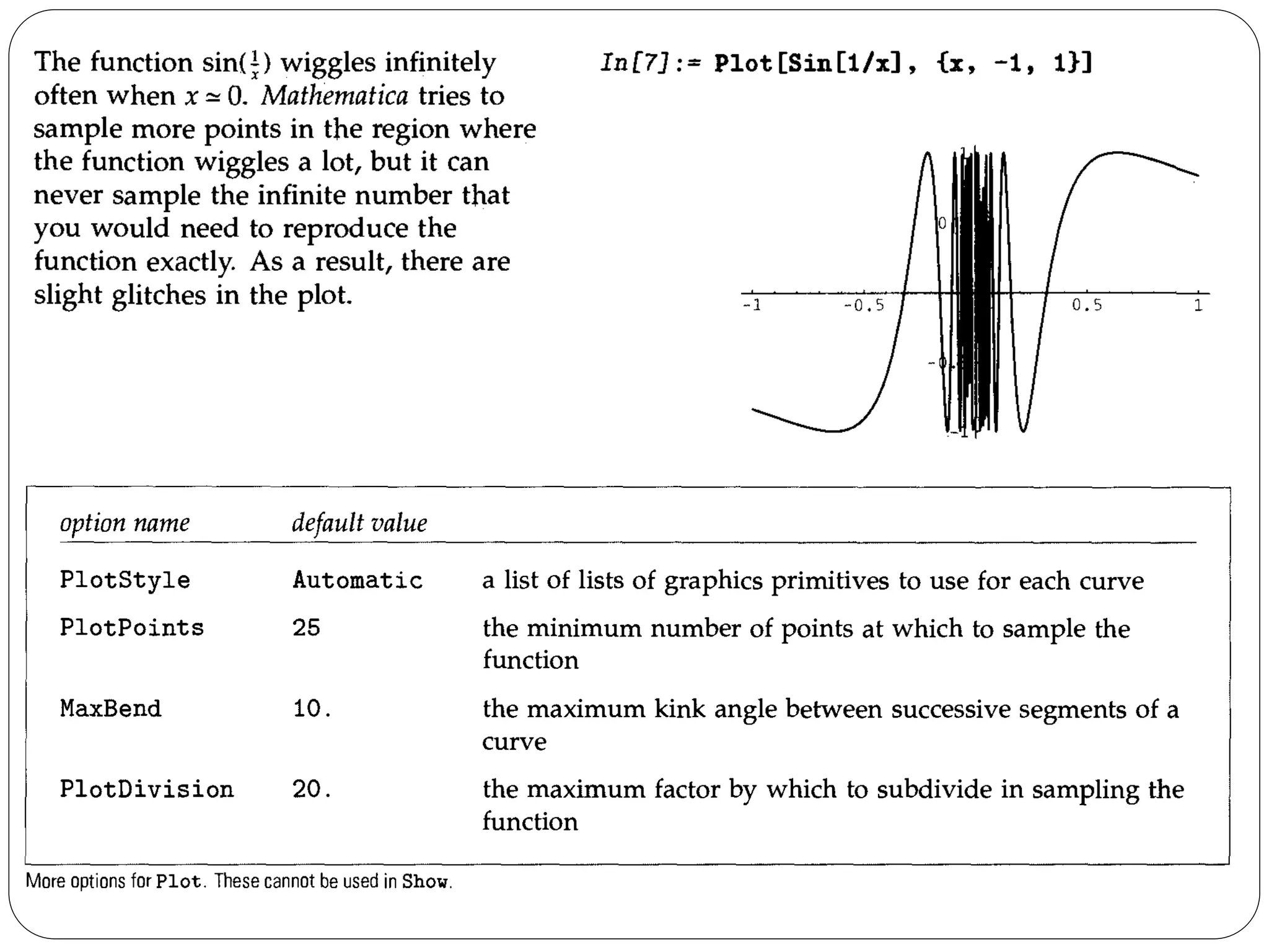
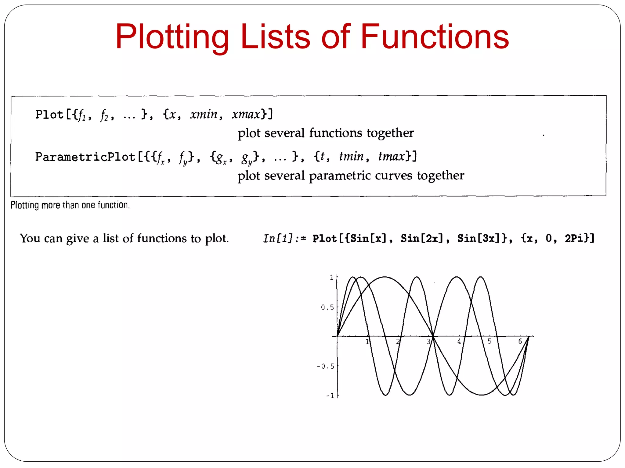
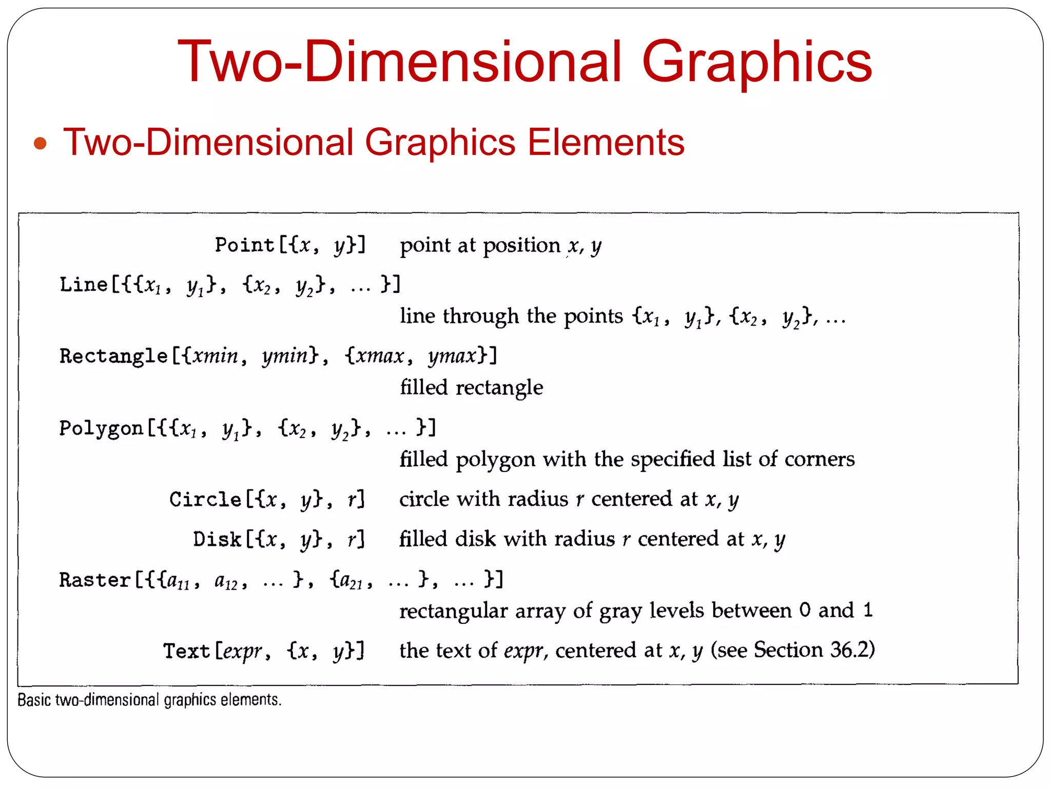
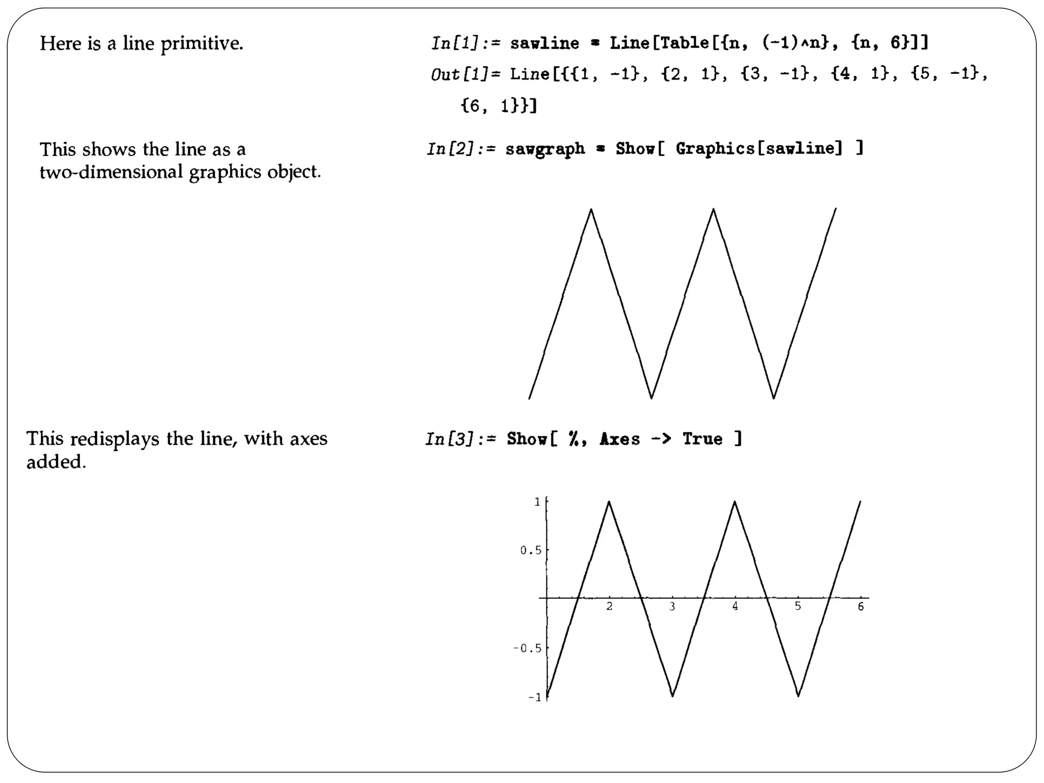
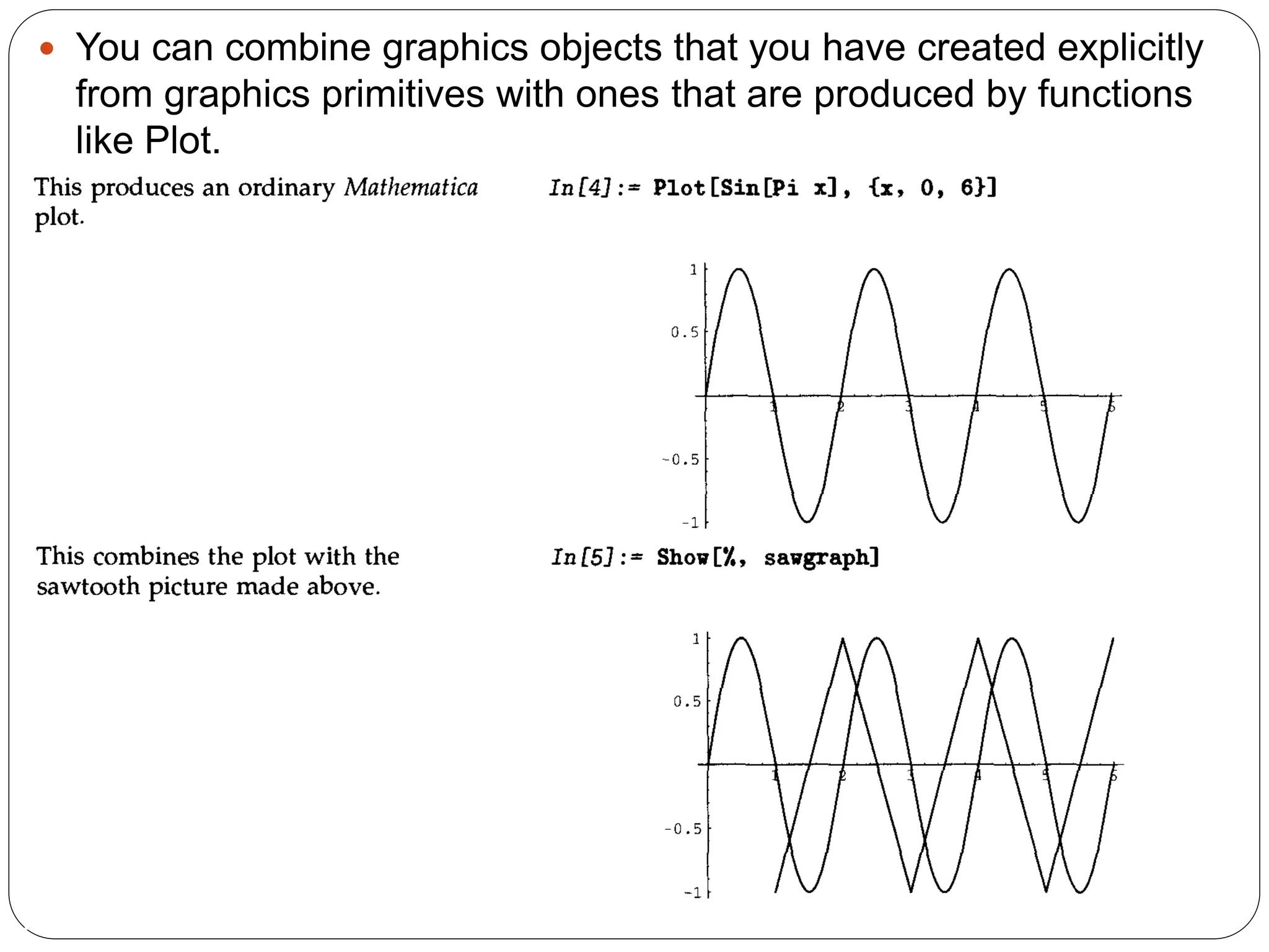
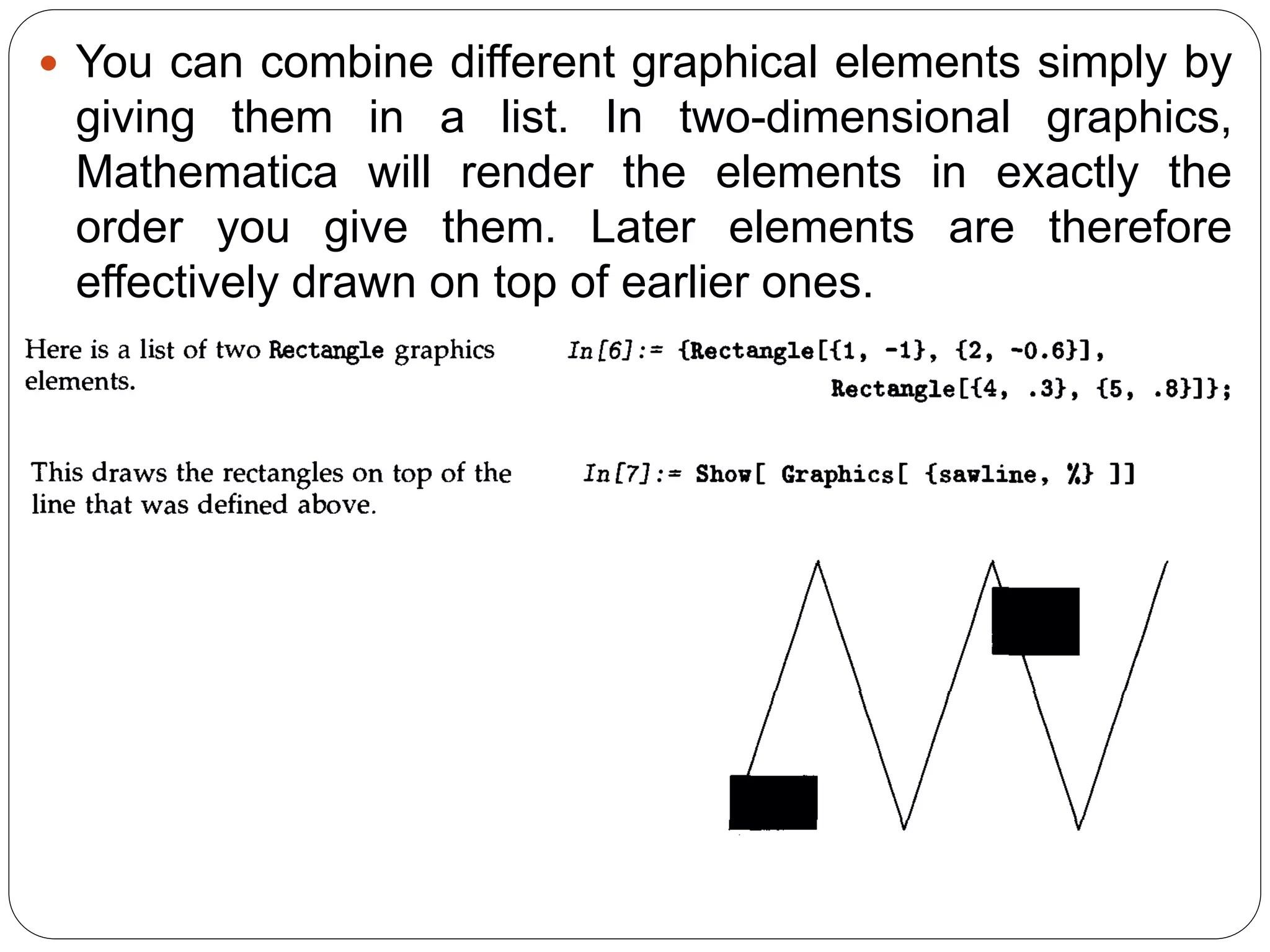
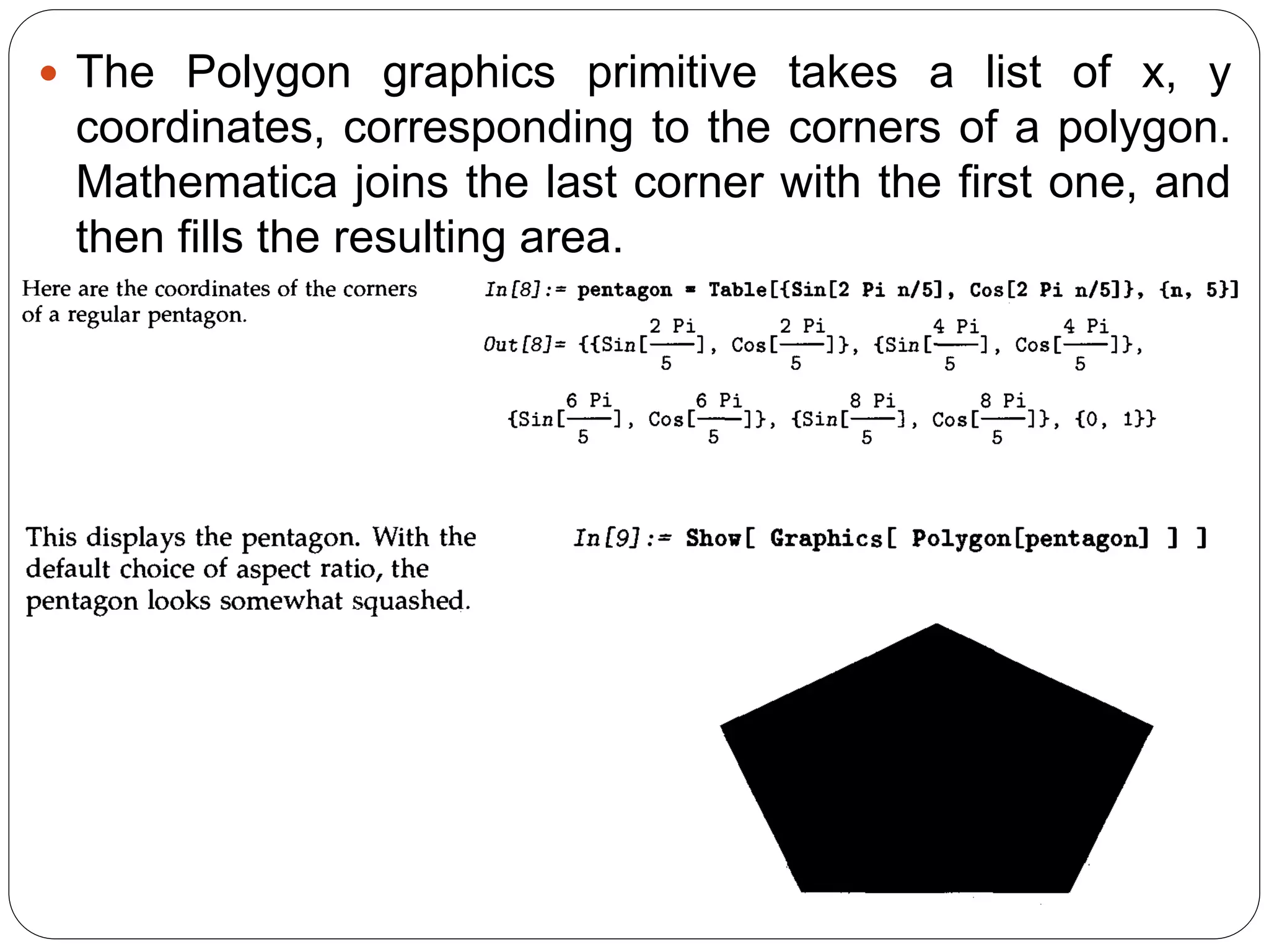
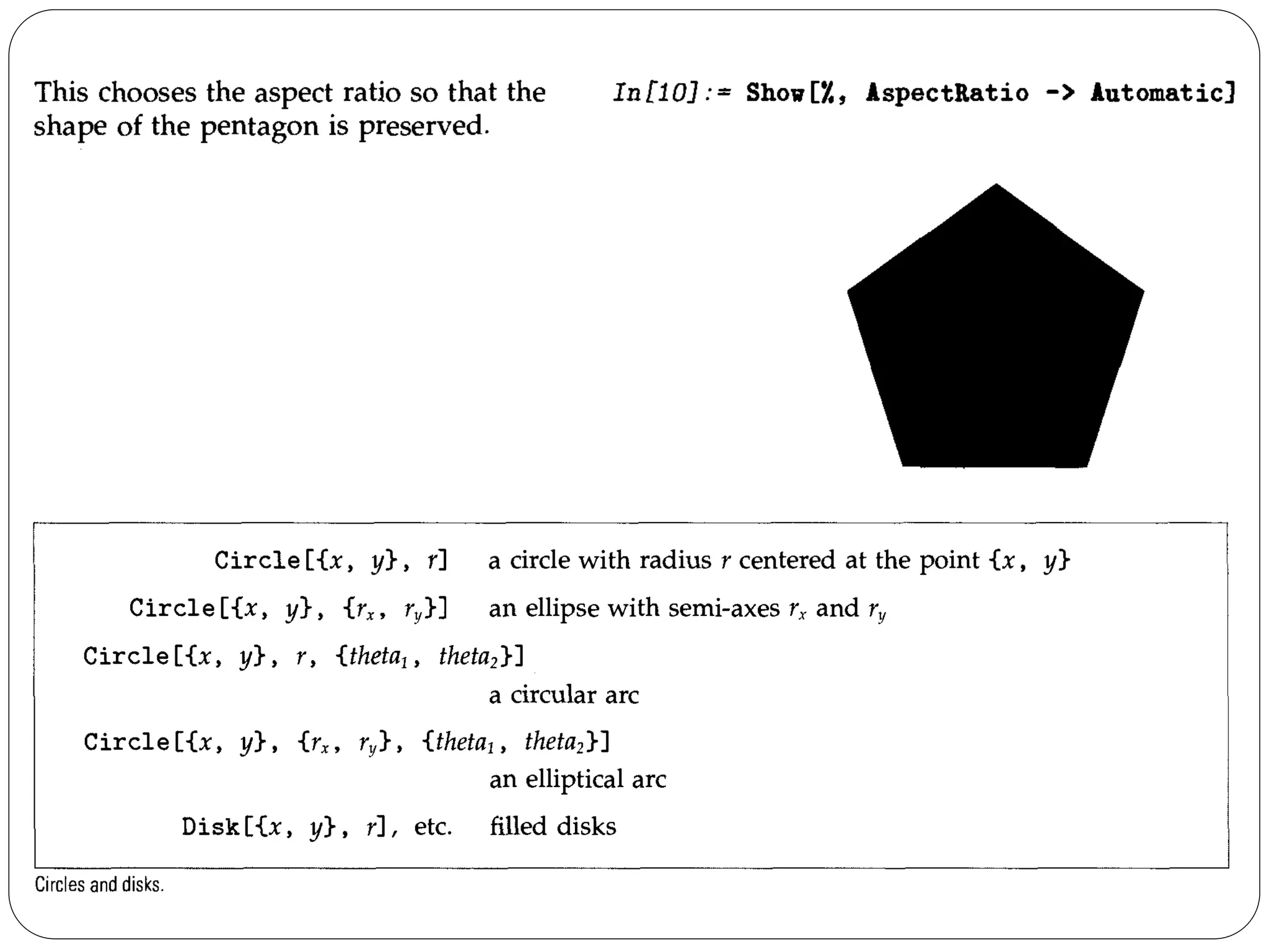
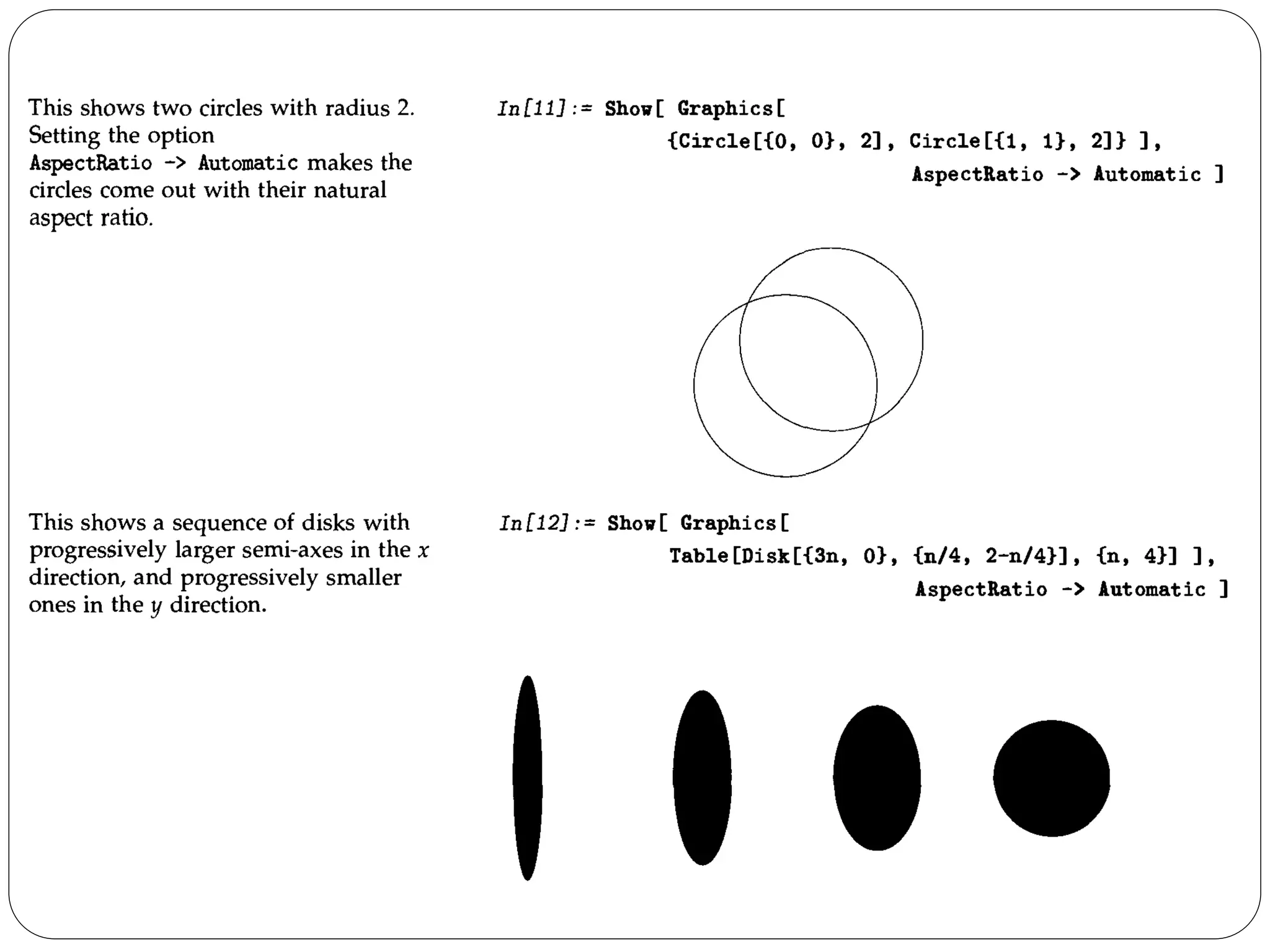
- The document discusses various plotting and graphics capabilities in Mathematica, including plotting functions, parametric plots, plotting lists of data, options for controlling plot appearance, and two-dimensional and three-dimensional graphics. - It describes how to control aspects of plots like scales, sampling of functions, and colors using options. It also covers various graphics primitives and directives for customizing plots.