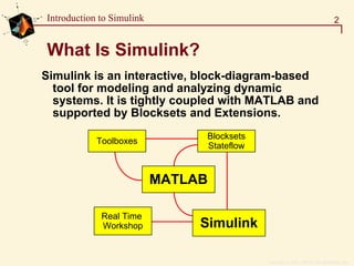
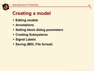
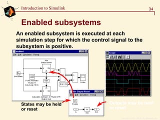
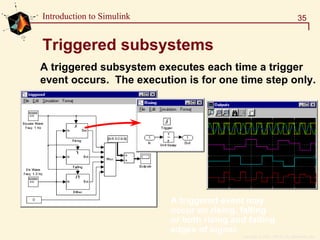
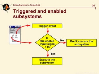
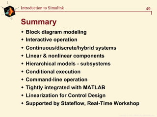
Simulink is an interactive block diagram modeling tool for dynamic systems that allows modeling of continuous, discrete, and hybrid systems. It provides nonlinear simulation capabilities and is tightly integrated with MATLAB for linearization, analysis of results, and control design. Models can contain hierarchical subsystems and support conditional execution.

1. Introduction to Simulink
Larry Michaels
michaels@mathworks.com
The MathWorks Inc.
24 Prime Park Way
Natick, MA 01760-1500
USA

2. Copyright  1984 - 1997 by The MathWorks, Inc.
2Introduction to Simulink
What Is Simulink?
Simulink is an interactive, block-diagram-based
tool for modeling and analyzing dynamic
systems. It is tightly coupled with MATLAB and
supported by Blocksets and Extensions.
Blocksets
Stateflow
Toolboxes
MATLAB
Real Time
Workshop Simulink

3. Copyright  1984 - 1997 by The MathWorks, Inc.
3Introduction to Simulink
What Is Simulink?
A simulation tool in MATLAB’s Technical
Computing Environment
Among other things, this means
Block diagram editing
Nonlinear simulation
Continuous and discrete simulation
Asynchronous (non-uniform sampling)
simulation
Integration with MATLAB, Extensions, Blocksets
& Toolboxes

4. Copyright  1984 - 1997 by The MathWorks, Inc.
4Introduction to Simulink
What can you model with
Simulink?
Just about anything you can model mathematically
Communications
and satellite
systems
Ship systems
Aircraft and spacecraft
dynamics and systems
Biological
systems
Monetary
systems
Automotive systems

5. Copyright  1984 - 1997 by The MathWorks, Inc.
5Introduction to Simulink
Building & Running a Model
Creating a model
Running the simulation
Analyzing the results

6. Copyright  1984 - 1997 by The MathWorks, Inc.
6Introduction to Simulink
Creating a model
Editing models
Annotations
Setting block dialog parameters
Creating Subsystems
Signal Labels
Saving (MDL File format)

7. Copyright  1984 - 1997 by The MathWorks, Inc.
7Introduction to Simulink
Open a new model window
Typing simulink
will also open a new
model window if no
other model is open
» simulink

8. Copyright  1984 - 1997 by The MathWorks, Inc.
8Introduction to Simulink
Collecting blocks
Pull the required
blocks into a new
SIMULINK block
diagram window.

9. Copyright  1984 - 1997 by The MathWorks, Inc.
9Introduction to Simulink
Connecting blocks
Left mouse
drag from
port to add
line
Right mouse drag to
add branch line

10. Copyright  1984 - 1997 by The MathWorks, Inc.
10Introduction to Simulink
Saving Model {
BlockDefaults {
}
AnnotationDefaults {
}
System {
Block
}
Line {
Branch {
}
}
}
}

11. Copyright  1984 - 1997 by The MathWorks, Inc.
11Introduction to Simulink
Creating Subsystems
Rename and save

12. Copyright  1984 - 1997 by The MathWorks, Inc.
12Introduction to Simulink
Annotations
Double click on
background
Type in the text

13. Copyright  1984 - 1997 by The MathWorks, Inc.
13Introduction to Simulink
Signal labels
Signal labels
work just like
annotations

14. Copyright  1984 - 1997 by The MathWorks, Inc.
14Introduction to Simulink
Signal labels
Signal labels can
pass through
"virtual" blocks

15. Copyright  1984 - 1997 by The MathWorks, Inc.
15Introduction to Simulink
Signal labels

16. Copyright  1984 - 1997 by The MathWorks, Inc.
16Introduction to Simulink
Vector I/O and Scalar Expansion
Vectorized
Inputs and
Outputs
Scalar
expansion of
parameter Wide Vector
Lines
Scalar
expansion of
inputs

17. Copyright  1984 - 1997 by The MathWorks, Inc.
17Introduction to Simulink
Defining variables
Both MATLAB and Simulink Windows “See” Into
the Same Workspace.
» x=21;
» t = 0:1
x=21
pi=3.14159...
t=[0 1]

18. Copyright  1984 - 1997 by The MathWorks, Inc.
18Introduction to Simulink
Goto / From blocks
Local [ ] is only
on the current
window

19. Copyright  1984 - 1997 by The MathWorks, Inc.
19Introduction to Simulink
Goto / From blocks
Global is all
systems

20. Copyright  1984 - 1997 by The MathWorks, Inc.
20Introduction to Simulink
Goto / From blocks
Tag
Visibility
is here
Scoped {} is all
systems
beneath the
Tag Visibility
block

21. Copyright  1984 - 1997 by The MathWorks, Inc.
21Introduction to Simulink
Running a simulation
Parameters dialog box
Continuous systems
Discrete systems
Getting data into models
From the command line

22. Copyright  1984 - 1997 by The MathWorks, Inc.
22Introduction to Simulink
Simulating
First simulation:
jagged!

23. Copyright  1984 - 1997 by The MathWorks, Inc.
23Introduction to Simulink
Setting parameters

24. Copyright  1984 - 1997 by The MathWorks, Inc.
24Introduction to Simulink
Simulating
Second
Simulation:
Much Better...
Use:
Variable-step discrete time solver
Max. Step Size = 0.1

25. Copyright  1984 - 1997 by The MathWorks, Inc.
25Introduction to Simulink
Setting parameters
h
t tstop start
max =
−
50

26. Copyright  1984 - 1997 by The MathWorks, Inc.
26Introduction to Simulink
Available Solvers
Variable-step solvers
Modify step size during simulation
Error control and zero crossing detection
ode45, ode23, ode113, ode15s, ode23s, discrete
Fixed-step solvers
Same step size throughout simulation
No error control or zero crossing detection
ode5, ode4, ode3, ode2, ode1, discrete
Simulink selects a default solver
ode45 used for models with continuous states
Variable-step discrete-time solver used for models
with no continuous states

27. Copyright  1984 - 1997 by The MathWorks, Inc.
27Introduction to Simulink
Getting data into and out of
models
Applies to
Inports and
Outports on top
level only

28. Copyright  1984 - 1997 by The MathWorks, Inc.
28Introduction to Simulink
Continuous models
Ordinary differential equations
F mx bx kx= + +
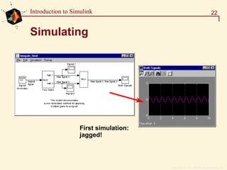
x
F
y
u ms bs k
= =
+ +
1
2
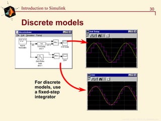
k
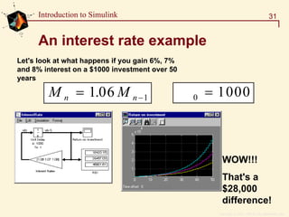
b
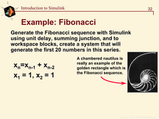
x(t)
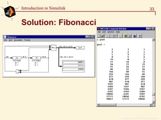
F(t)
m
[m b k]

29. Copyright  1984 - 1997 by The MathWorks, Inc.
29Introduction to Simulink
Spring-Mass-Damper

30. Copyright  1984 - 1997 by The MathWorks, Inc.
30Introduction to Simulink
Discrete models
For discrete
models, use
a fixed-step
integrator

31. Copyright  1984 - 1997 by The MathWorks, Inc.
31Introduction to Simulink
An interest rate example
Let's look at what happens if you gain 6%, 7%
and 8% interest on a $1000 investment over 50
years
M Mn n= −1 06 1. M 0 1000=
WOW!!!
That's a
$28,000
difference!

32. Copyright  1984 - 1997 by The MathWorks, Inc.
32Introduction to Simulink
Example: Fibonacci
xxnn==xxnn--11 ++ xxnn--22
xx11 = 1, x= 1, x22 = 1= 1
Generate theGenerate the FibonacciFibonacci sequence withsequence with SimulinkSimulink
using unit delay, summing junction, and tousing unit delay, summing junction, and to
workspace blocks, create a system that willworkspace blocks, create a system that will
generate the first 20 numbers in this series.generate the first 20 numbers in this series.
A chambered nautilus is
really an example of the
golden rectangle which is
the Fibonacci sequence.

33. Copyright  1984 - 1997 by The MathWorks, Inc.
33Introduction to Simulink
Solution: Fibonacci

34. Copyright  1984 - 1997 by The MathWorks, Inc.
34Introduction to Simulink
Enabled subsystems
An enabled subsystem is executed at each
simulation step for which the control signal to the
subsystem is positive.
Outputs may be held
or reset
States may be held
or reset

35. Copyright  1984 - 1997 by The MathWorks, Inc.
35Introduction to Simulink
Triggered subsystems
A triggered subsystem executes each time a trigger
event occurs. The execution is for one time step only.
A triggered event may
occur on rising, falling
or both rising and falling
edges of signal.

36. Copyright  1984 - 1997 by The MathWorks, Inc.
36Introduction to Simulink
Triggered and enabled
subsystems
Trigger event
Is
the enable
input signal
> 0?
No Don't execute the
subsystem
Yes
Execute the
subsystem

37. Copyright  1984 - 1997 by The MathWorks, Inc.
37Introduction to Simulink
From the command line
Why simulate from the command line?
Automate repeated simulations
Parameter tuning
Parameter Optimization (NCD)

38. Copyright  1984 - 1997 by The MathWorks, Inc.
38Introduction to Simulink
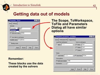
From the command line
(The most basic method)
[t,x,y]=sim(model)
[t,x,y1,y2,…, yn]=sim(model)
Simulates the model using all of the model
parameters.
The time, state and output vectors are returned
from the simulation.
Individual outputs may be obtained.
Outputs are obtained from the outport blocks on
the top level of the model.

39. Copyright  1984 - 1997 by The MathWorks, Inc.
39Introduction to Simulink
From the command line
» options=simget('external_pendulum')
options =
Solver: 'ode45'
RelTol: 1.0000e-003
AbsTol: 1.0000e-006
Refine: 1
MaxStep: 0.1000
InitialStep: 'auto'
MaxOrder: 5
FixedStep: 'auto'
OutputPoints: 'all'
OutputVariables: ''
MaxRows: 1000
Decimation: 1
InitialState: []
FinalStateName: 'xFinal'
Debug: 'off'
Trace: ''
SrcWorkspace: 'current'
DstWorkspace: 'current'
ZeroCross: 'on'
Use simget and simset to
get and set the options
structure.
[t,x,y]=sim(model, timespan, options)
options is a data
structure that contains
all of the solver
parameters
The options structure
overrides the simulation
parameters settings

40. Copyright  1984 - 1997 by The MathWorks, Inc.
40Introduction to Simulink
From the command line
[t,x,y]=sim(model, timespan, options, ut)
ut allows external inputs to be supplied to the inports
on the top level of the model.
[] in place of timespan or options indicates that the
current model settings are used.

41. Copyright  1984 - 1997 by The MathWorks, Inc.
41Introduction to Simulink
Analyzing results
Getting data out of models
Floating Scope and Display blocks
Trim
Linearization

42. Copyright  1984 - 1997 by The MathWorks, Inc.
42Introduction to Simulink
Getting data out of models
The Scope, ToWorkspace,
ToFile and Parameters
Dialog all have similar
options
Remember:
These blocks use the data
created by the solvers

43. Copyright  1984 - 1997 by The MathWorks, Inc.
43Introduction to Simulink
The floating Scope and Display
blocks
Selecting any signal will
display the value(s) of that
signal on any floating
scope or display block on
that diagram
Unselected

44. Copyright  1984 - 1997 by The MathWorks, Inc.
44Introduction to Simulink
The floating Scope and Display
blocks
Selected

45. Copyright  1984 - 1997 by The MathWorks, Inc.
45Introduction to Simulink
The floating Scope and Display
blocks
You can even select multiple signals...
Selected

46. Copyright  1984 - 1997 by The MathWorks, Inc.
46Introduction to Simulink
Trim
Find the values of states x and inputs u that
bring the system to steady state (dx=0)
The solution is not necessarily unique
[x, u, y]=trim('sys')
To provide an initial guess at the solution
[x, u, y]=trim('sys', x0, u0, y0)
Individual elements of x,u,y can be constrained
Individual derivatives can be fixed to non-zero
values
Can also add a fourth output argument to get the
state derivatives at trim ([x,u,y,dx]=…)

47. Copyright  1984 - 1997 by The MathWorks, Inc.
47Introduction to Simulink
Linearization
Use linmod to extract linear models from
Simulink systems
Perturbs each state around the operating point to
determine the rate of change in the state
derivatives and outputs (Jacobians)
Use linmod2 for advanced linearization
attempts to balance roundoff and truncation error
perturbation levels of each state-space matrix
element set individually
can detect discontinuities and produce warning
messages

48. Copyright  1984 - 1997 by The MathWorks, Inc.
48Introduction to Simulink
Discrete linearization - dlinmod
Used for discrete, multi-rate and hybrid systems
One additional input argument, Ts, after the
system name
[Ad, Bd, Cd, Dd]=dlinmod('sys',Ts,x,u)
Use Ts=0 for a continuous model approximation

49. Copyright  1984 - 1997 by The MathWorks, Inc.
49Introduction to Simulink
Summary
Block diagram modeling
Interactive operation
Continuous/discrete/hybrid systems
Linear & nonlinear components
Hierarchical models - subsystems
Conditional execution
Command-line operation
Tightly integrated with MATLAB
Linearization for Control Design
Supported by Stateflow, Real-Time Workshop