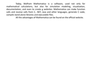
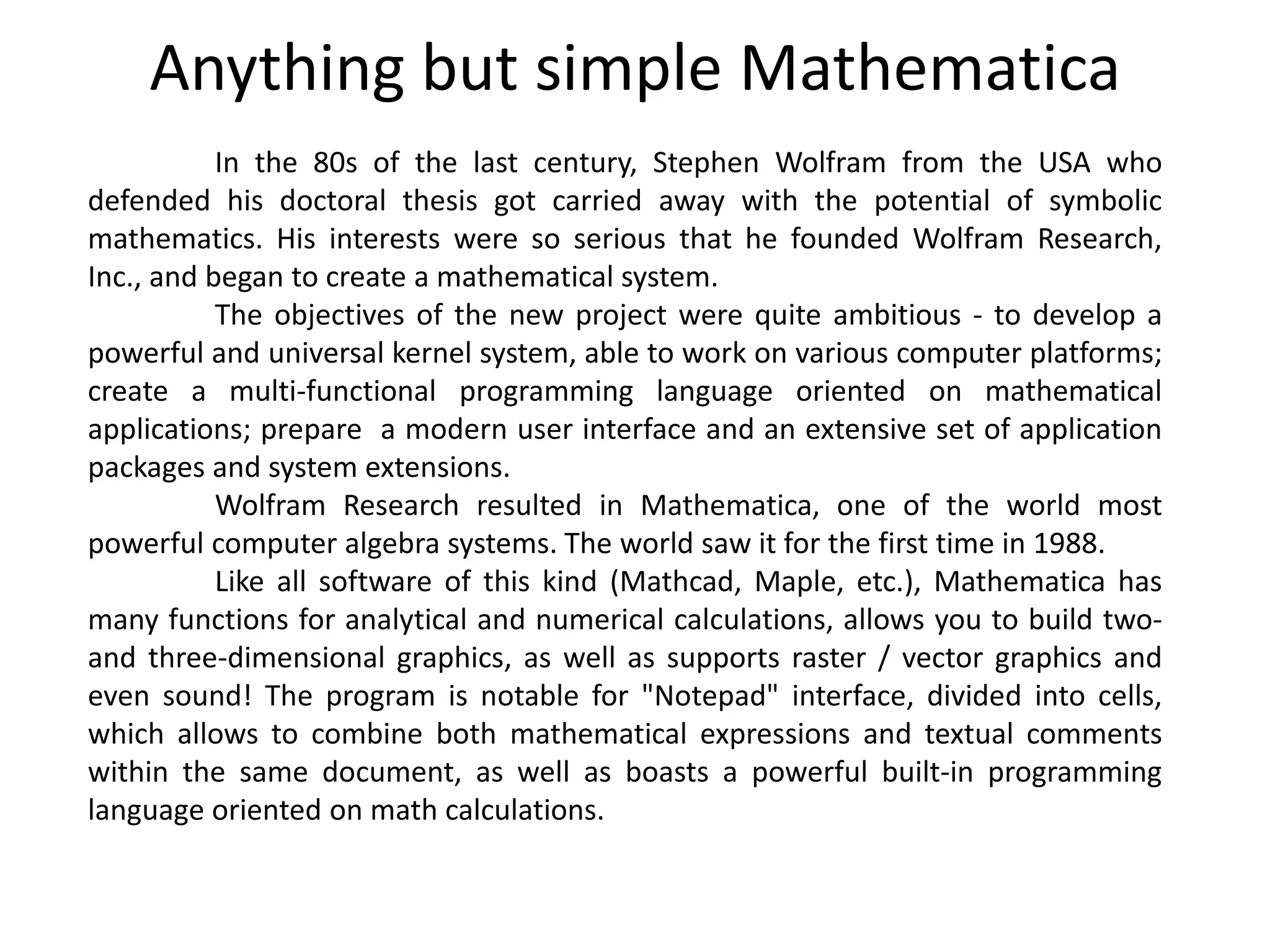
Wolfram Research created Mathematica, one of the most powerful computer algebra systems, to fulfill Stephen Wolfram's vision of a universal mathematical kernel. Mathematica allows analytical and numerical calculations, 2D and 3D graphics, and includes a powerful programming language. While initially designed for mathematical applications, Mathematica is now used for simulation, modeling, visualization, documentation, and more.

1. Anything but simple Mathematica
In the 80s of the last century, Stephen Wolfram from the USA who
defended his doctoral thesis got carried away with the potential of symbolic
mathematics. His interests were so serious that he founded Wolfram Research,
Inc., and began to create a mathematical system.
The objectives of the new project were quite ambitious - to develop a
powerful and universal kernel system, able to work on various computer platforms;
create a multi-functional programming language oriented on mathematical
applications; prepare a modern user interface and an extensive set of application
packages and system extensions.
Wolfram Research resulted in Mathematica, one of the world most
powerful computer algebra systems. The world saw it for the first time in 1988.
Like all software of this kind (Mathcad, Maple, etc.), Mathematica has
many functions for analytical and numerical calculations, allows you to build two-
and three-dimensional graphics, as well as supports raster / vector graphics and
even sound! The program is notable for "Notepad" interface, divided into cells,
which allows to combine both mathematical expressions and textual comments
within the same document, as well as boasts a powerful built-in programming
language oriented on math calculations.

2. What is Mathematica all about?
Run the program, and a large white window - a notebook will appear on
the screen on the left. This is where the information is entered and the results are
displayed. The window in the middle is a welcome screen saver. Toolbars can be
displayed on the right.
Switch to Notepad and enter the following expression (command):
2 + 8
To calculate, you need to press "Shift + Enter" (or "Enter" on the numeric
keypad). Once calculations are done, you can see the original expression and the
answer on the screen:
In[1]: = 2 + 8
Out[1] = 10
The original expression is assigned as a value to the "In[1]" object, while
the result to the "Out[1]" object. These objects appear after the calculation, so do
not expect prompting "In[2]: =" to enter the next expression.
In addition, you can see square brackets appear along the right side of
the notebook. The original expression and the result are enclosed in cells, which
are bounded by these very square brackets. Each such pair of I/O is enclosed, in
turn, in a grouping bracket combining both the original expression and the result.
By Selecting the bracket limiting a cell and doing a right mouth click , you
can call a context menu and select Style in it. Here you can see the cell formatting
styles. We are interested in Input only- it serves for data entry and is used by
default in each new input cell; while the Text style is used for text notes and
comments thus being completely ignored during the calculation.

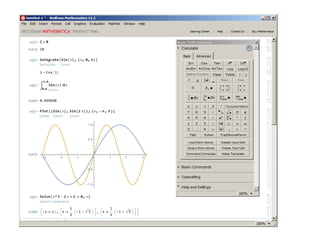
3. Let's try to calculate the indefinite integral of the function sin(x). To do
this, find “Palettes > Basic Math Assistant> Calculator” toolbar, click “Advanced”
tab, and find indefinite integral “∫□d□“ icon, then enter the Sin[x] function to end
up with ∫Sin[x]dx, or you can simply type “Integrate[Sin[x],x]”. It worth mentioning
that you should use square brackets [] to enter the function arguments. Bear in
mind that the program differentiates between lowercase and uppercase letters, so
you cannot enter sin or SIN instead of Sin.
To calculate a specific integral, either click the corresponding button on
the toolbar, or add the integration limits in curly brackets:
In[3]: = Integrate[Sin[x],{x,0,1}]
Out[3] = 1-Cos[1]
For Mathematica to give an answer straightaway in a numerical form, it is
necessary to use the real number format, characterized by a fractional point.
In[4]: = Integrate[Sin[x],{x,0.,1.}]
Out[4] = 0.459698
Moreover, using curly brackets, it is easy to build graphs of several
functions within one figure, for example, sin(x) and sin(2x):
Plot[{Sin[x],Sin[2x]},{x,-π,π}]
there are more than 20 options defining styles and additional graph elements
catering to a better display.

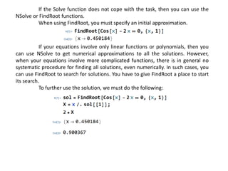
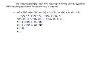
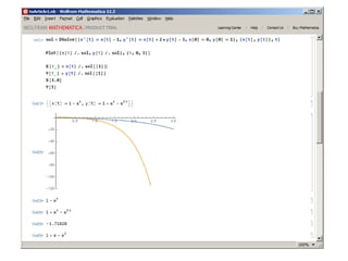
5. Solving the equation in Mathematica is also a snap. Suppose you need to
find the roots of the equation x^3 - 2x +1 = 0. This is easy and simple:
In this case, the answer is given in integers, which sometimes makes it
difficult to have an idea of the resulted magnitude. To have the answer displayed
as a floating point number, do the following:
N[Solve [x ^ 3-2x + 1 == 0, x]] or
Solve[x ^ 3-2x + 1 == 0, x] // N
The function N[expr] - displays the numerical value of the expression expr.
As a result, in both cases the following will be displayed:
{{x → 1.}, {x → -1.618033988749895}, {x → 0.6180339887498949}}
To solve the system of equations, the Solve function is also used:

6. If your equations involve only linear functions or polynomials, then you
can use NSolve to get numerical approximations to all the solutions. However,
when your equations involve more complicated functions, there is in general no
systematic procedure for finding all solutions, even numerically. In such cases, you
can use FindRoot to search for solutions. You have to give FindRoot a place to start
its search.
To further use the solution, we must do the following:
If the Solve function does not cope with the task, then you can use the
NSolve or FindRoot functions.
When using FindRoot, you must specify an initial approximation.

7. Like any earnest computer algebra Mathematica allows to solve
differential equations and then use the results for further calculations.
Find the general solution of the ordinary first order differential equation
y '- ax = 0
We solve the same equation for a = 3 and for y (0) = 1;
Or a system of differential equations:

8. The following example shows how the program having solved a system of
differential equations uses further the results obtained

10. Mathematica is an extensible system. In addition to the internal
Mathematica core commands, you can use additional commands to be found in
the loaded packages. Some system packages (for algebra, analysis, etc.) are
supplied with the program itself and are standard. Other packages can be
downloaded from Wolfram Research’s server or purchased separately.
The Mathematica extension packages (Add-ons) are sets of files with the
.m extension, written in the system programming language and combined under
the names of the corresponding packages. Packages add to the system a number of
functions that are missing in the system kernel They can be easily modified and
created, so that you can easily adapt the system for specific tasks.
To execute a command from the Mathematica package, you must first
load the required package using the << dir'package 'or << dir command. The last
command initializes all the packages from the dir folder. Here's how, for example,
you can initialize all algebraic packages: << Algebra ', while connecting the package
<< Units' allows you to convert units of measure of various physical quantities.

11. Everything above mentioned concerned using Mathematica system to solve
mathematical tasks. However, this does not mean at all that, if necessary, Mathematica
cannot be used for simple or complex programming, for which the existing built-in
functions and even extension packages are not enough or that require software tools
inherent in ordinary programming languages to implement their algorithms. Everything
is completely different.
Here are some features provided by Mathematica for writing programs:
• Cycle Organization
• Conditional expressions and unconditional transfers
• User functions
• Patterns and their use
• Use of procedures
• FixedPoint and Catch functions
• Implementation of recursive and recurrent algorithms
• Preparation of extension packs
• Visual programming tools
• Program Debugging and tracing.

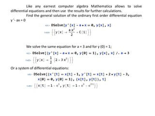
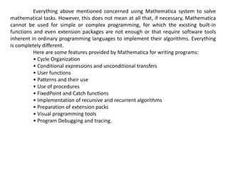
12. In fact, Mathematica is based on an ultra-high level mathematical
problem-oriented programming language.
Below is a listing written in the Mathematica programming language. I
think no comments are needed
In[11]:=For [ i = 1, i<=3, Print ["Hello World!"]; i + + ]
Hello World!
Hello World!
Hello World!
It is important to emphasize that here we are talking about the
programming language of the Mathematica, and not about its implementation
language. The system is implemented in C ++, which has shown its high efficiency
as a system programming language.

13. Today, Wolfram Mathematica is a software, used not only for
mathematical calculations, but also for simulation modeling, visualization,
documentation, and even to create g websites. Mathematica can make function
calls and receive calls from C, .NET, Java and other languages, generate C code,
compile stand-alone libraries and executable files.
All the advantages of Mathematica can be found on the official website.