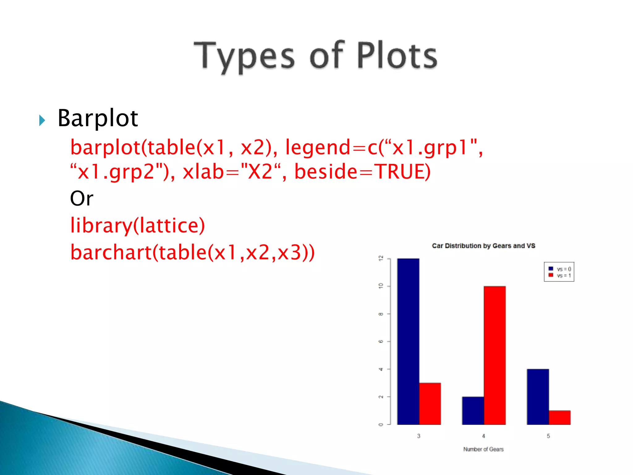
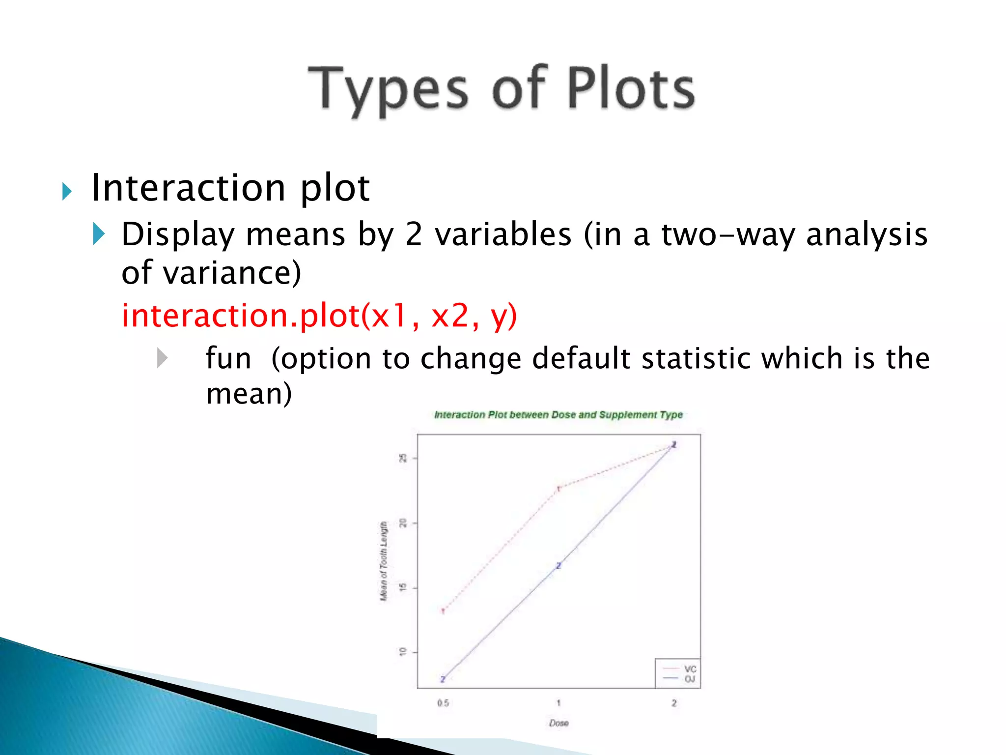
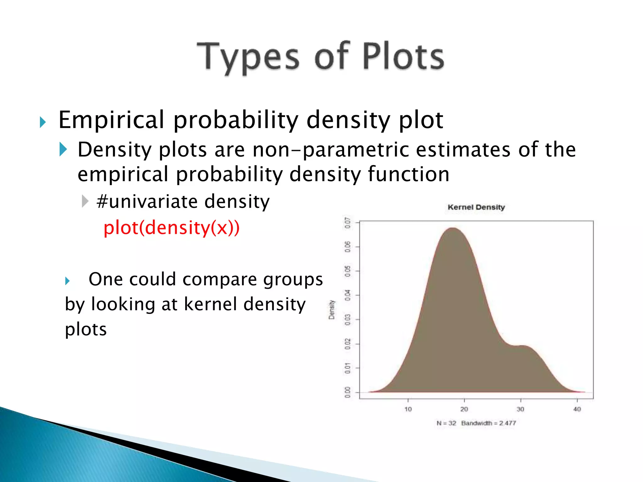
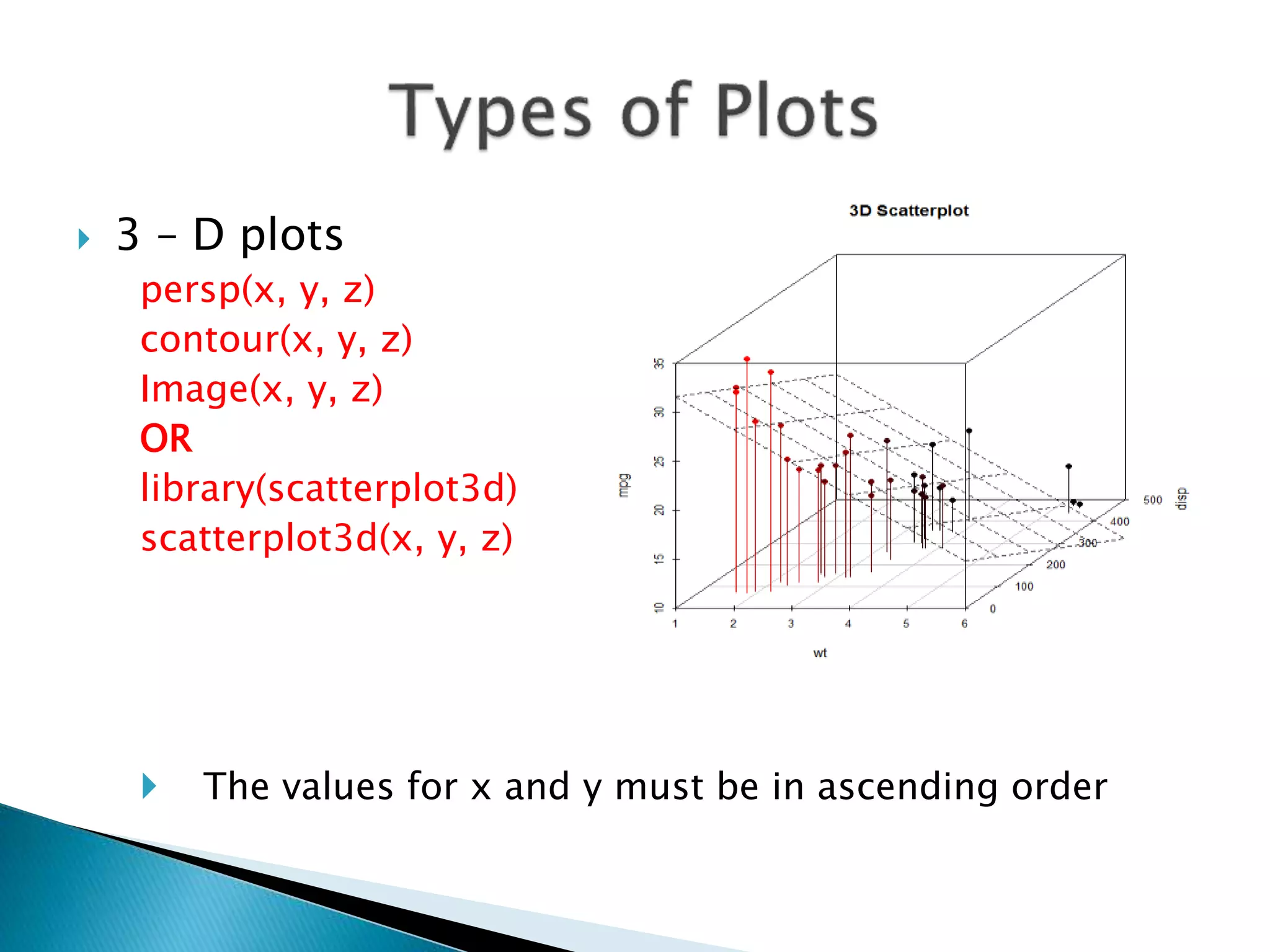
This document provides an overview of various plotting functions in R for visualizing data including quantile-quantile plots, barplots, boxplots, interaction plots, density plots, 3D plots, and adjusting graphical parameters such as colors, sizes, fonts and saving plots. Key functions discussed are qqnorm, qqline, barplot, boxplot, interaction.plot, density, persp, contour, par, and devices like pdf, jpeg for saving plots.

2.  Quantile-quantile plots
qqnorm(x)
qqline(x)
Quantile – Quantile-Quantile plot
qqplot(x, y)

3.  Barplot
barplot(table(x1, x2), legend=c(“x1.grp1",
“x1.grp2"), xlab="X2“, beside=TRUE)
Or
library(lattice)
barchart(table(x1,x2,x3))

4.  Boxplots and Violin Plots
boxplot(x)
 horizontal = TRUE
library(vioplot)
vioplot(x1, x2, x3)
• Side-by-side boxplots
boxplot(y~x)
Or
library(lattice)
bwplot(y~x)

5.  Interaction plot
 Display means by 2 variables (in a two-way analysis
of variance)
interaction.plot(x1, x2, y)
 fun (option to change default statistic which is the
mean)

6.  Empirical probability density plot
 Density plots are non-parametric estimates of the
empirical probability density function
 #univariate density
plot(density(x))
 One could compare groups
by looking at kernel density
plots

7.  3 – D plots
persp(x, y, z)
contour(x, y, z)
Image(x, y, z)
OR
library(scatterplot3d)
scatterplot3d(x, y, z)
 The values for x and y must be in ascending order

8.  A list of graphical parameters that define the
default behavior of all plot functions.
 Just like other R objects, par elements are similarly
modifiable, with slightly different syntax.
◦ e.g. par(“bg”=“lightcyan”)
◦ This would change the background color of all
subsequent plots to light cyan
 When par elements are modified directly (as above,
this changes all subsequent plotting behavior.

9.  Size of margins
◦ par(mar=c(bot, left, top, right))
 Save graphical settings
◦ par() #view currents settings
◦ opar <- par() #make a copy of current settings
◦ par(opar) #restore original settings
 Multiple plots per page
◦ par(mfrow=c(a, b)) #a rows and b columns
◦ par(mfcol=c(a,b))

10.  bg – plot background color
 lty – line type (e.g. dot, dash, solid)
 lwd – line width
 col – color
 cex – text size inside plot
 xlab, ylab – axes labels
 main – title
 pch – plotting symbol

11.  Add an arbitrary straight line:
 plot(x, y)
 abline(intercept, slope)
 Plot symbols
 plot(x, y, pch=pchval)
PCH symbols used in R
 “col=“ and “bg=” are also specified
 PCH can also be in characters such as
“A”, “a”, “%” etc.

12.  Titles
 title(main=“main” , sub = “sub”, xlab=“xlab”, ylab=“ylab”)
 Mathematical Symbols
 plot(x, y)
 expr = expression(paste(mathexpression)))
 title(xlab=c(expr))
 Arrows and Shapes
 arrows(x, y)
 rect(xleft, ybottom, xright, ytop)
 polygon(x, y)
 library(plotrix)
 draw.circle(x, y, r)

14.  Line styles, line width and colors
 plot(….)
 lines(x, y, lty=ltyval, lwd = lwdval,
col=colval)
col Default plotting color. Some functions (e.g. lines)
accept a vector of values that are recycled.
col.axis color for axis annotation
col.lab color for x and y labels
col.main color for titles
col.sub color for subtitles
fg plot foreground color (axes, boxes - also sets col= to
same)
bg plot background color

15.  Legend
 plot(x, y)
 legend(xval, yval, legend = c(“Grp1”, “Grp2”),
lty=1:2, col=3:4, bty=“box type”)
 Add a legend at the location at (xval, yval)
 A vector of legend labels, line types,
and colors can be specified
using legend, lty and col options.
 bty =“o” or “n”

16.  Adding Points or Lines to an Existing Graphic
 plot(x, y)
 points(x, y)
 lines(x, y, type=“type”)
type =
 p points
 l lines
 o overplotted points and lines
 b, c points (empty if "c") joined by lines
 s, S stair steps
 h histogram-like vertical lines
 n does not produce any points or lines
 OLS line fit to the points
 plot(x, y)
 abline(lm(y~x))

17.  Graph Size
 pdf(“filename.pdf”, width = Xin, height = Yin)
 Point and text size
 plot(x, y, cex = cexval)
 cex number indicating the amount by which
plotting text and symbols should be scaled relative to the
default. 1=default, 1.5 is 50% larger, 0.5 is 50% smaller,
etc.
 cex.axis magnification of axis annotation relative to cex
 cex.lab magnification of x and y labels relative to cex
 cex.main magnification of titles relative to cex
 cex.sub magnification of subtitles relative to cex
 Box around plots
 plot(x, y, bty = btyval)

18.  Axis labels, values, and tick marks
◦ plot(x, y, lab=c(x, y, len), #number of tick marks
las=lasval, #orientation of tick marks
tck = tckval, #length of tick marks
xaxp = c(x1, x2, n), #coordinates of the extreme tick
marks
yaxp = c(x1, x2, n),
xlab = “X axis label”, ylab=“Y axis label”)
◦ las = 0 labels are parallel to axis
◦ las=2 labels are perpendicular to axis
◦ tck = 0 suppresses the tick mark

19.  Axis Range and Style
◦ plot(x, y, xlim = c(minx, maxx), ylim = c (miny, maxy),
xaxs=“i”, yaxs=“i”)
 The xaxs and yaxs control whether the tick marks extend
beyond the limits of the plotted observations (default) or are
constrained to be internal (“i”)
 See also:
 axis()
 mtext()
 Omit axis
◦ plot(x, y, xaxt = “n”, yaxy=“n”)

20.  Fonts
 font Integer specifying font to use for text.
1=plain, 2=bold, 3=italic, 4=bold italic,
5=symbol
 font.axis font for axis annotation
 font.lab font for x and y labels
 font.main font for titles
 font.sub font for subtitles
 ps font point size (roughly 1/72 inch)
text size=ps*cex
 family font family for drawing text. Standard values
are "serif", "sans", "mono", "symbol".

21.  More on how to change colors
◦ You can specify colors in R by index, name,
hexadecimal, or RGB.
◦ For example col=1, col="white", and col="#FFFFFF"
are equivalent.
◦ colors() #list of color names

22.  The number of plots on a page, and their placement on the page,
can be controlled using par() or layout().
 The number of figure regions can be controlled using mfrow and
mfcol.
e.g. par(mfrow=c(3,2)) # Creates 6 figures arranged in
3 rows and 2 columns
 layout() allows the creation of multiple figure regions of unequal
sizes.
e.g. layout(matrix(c(1,2)), heights=c(2,1))

23.  Many statistical functions (regression, cluster
analysis) create special objects. These arguments
will automatically format graphical output in a
specific way.
 e.g. Produce diagnostic plots from a linear model
analysis (see R code)
# Reg = lm()
# plot(Reg)
 hclust()
 agnes() # hierarchical cluster analysis

24.  Specify destination of graphics output or simply right
click and copy
 Could be files
◦ Not Scalable
 JPG # not recommended, introduces blurry artifacts
around the lines
 BMP
 PNG
◦ Scalable:
 Postscript # preferred in LaTex
 Pdf # great for posters

25.  pdf(“file.pdf”)
 plot(….)
 dev.off()
 jpeg(“file.jpeg”)
 plot(…)
 dev.off()
 win.metafile(file.wmf)
 plot(…)
 dev.off()
 Similar code for BMP, TIFF, PNG, POSTSCRIPT
 PNG is usually recommended
 The dev.off() function is used to close the graphical device