This document discusses using Mathematica software for computational learning at St John's Anglican College. It has been used with senior mathematics students for the past five years, starting with Year 11 classes and expanding to all year levels 7-12. Mathematica allows students to model and solve computational problems, developing complex solutions. It also enables interactive notebooks with executable code and functions. Students use Mathematica for a range of tasks from basic computations to modeling more complex real-life situations. An example is provided of using Mathematica to determine the line of best fit for sunflower height data over time using a logistic model.
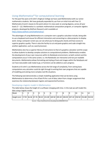
![Using Mathematica students are first able to enter the data into a variable, called data:
The text that follows the “In[#]:=” is what is entered by the user and the “Out[#]:=” is followed by
the output that Mathematica produces in response.
The data can then be modelled by any function, as specified by the function FindFit. This example
below generates values for the parameters 𝑐𝑐, 𝑑𝑑 and 𝑟𝑟 with the independent variable being 𝑡𝑡. The
natural number ‘e’ can be represented in Mathematica as either a capital ‘E’ or the ‘e’ used below
which is available from the palettes menu.
These values can then be substituted into the function and plotted, but one handy feature of
Mathematica is that it provides some likely next steps. In this case we can select plot fit from the
context menu that appears below the output line, as circled above.
This produces the relevant code to show the line of best fit and the data on the same graph:
Larger data sets can be imported
directly into Mathematica from a
delimited text file or csv.
Variables in Mathematica are very
easy to work with as they don’t need
to be declared or defined previously.](https://image.slidesharecdn.com/acdefeab-25a6-4d33-8175-adc71dea96d0-160227135038/85/Using-Mathematica-for-computational-learning-2-320.jpg)
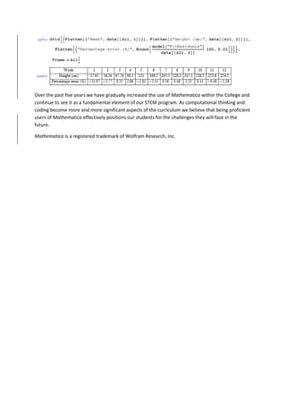
![We can also use a different function called NonlinearModelFit if we’re interested in doing some
further analysis. In this example the model is stored to a variable simply called model:
We can present the function as either the equation or the parameters determined:
We can examine the accuracy of our model to the original data:
We can use these results to then work out other values, such as the percentage errors:
This takes the “FitResiduals” values of model and divides each by the original value from data, then
multiplies by 100. The instruction - data[[All, 2]] - tells Mathematica to get all the values from the
second column of data.
In this demonstration I’ve focused primarily on the calculation side of Mathematica, but as
mentioned in the beginning it also has graphical and presentation features that can be utilised to
produce a more visually pleasing product. The following code presents the data generated earlier in
a table format:
These are three examples of over
forty properties that can be
examined directly.](https://image.slidesharecdn.com/acdefeab-25a6-4d33-8175-adc71dea96d0-160227135038/85/Using-Mathematica-for-computational-learning-3-320.jpg)