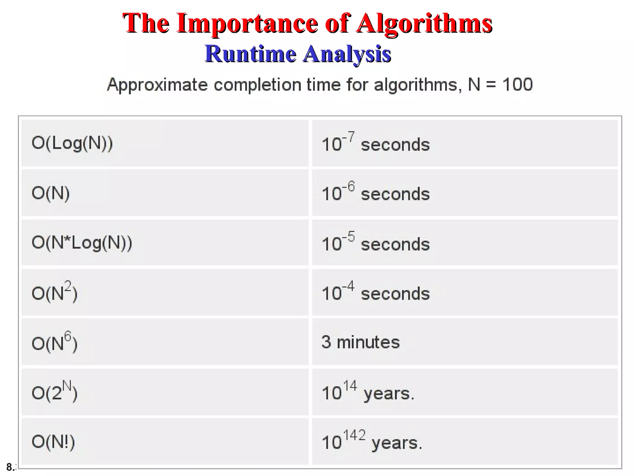
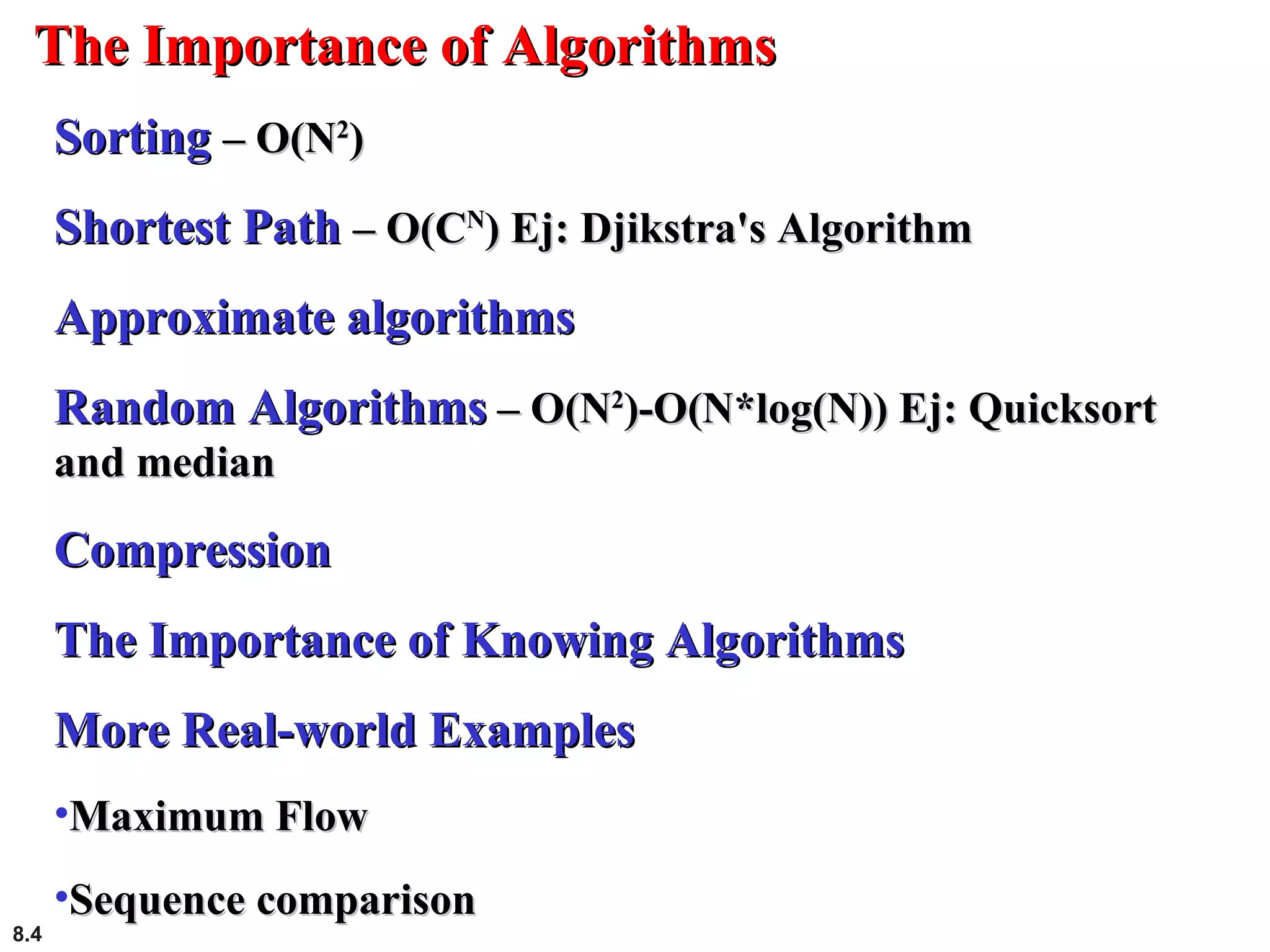
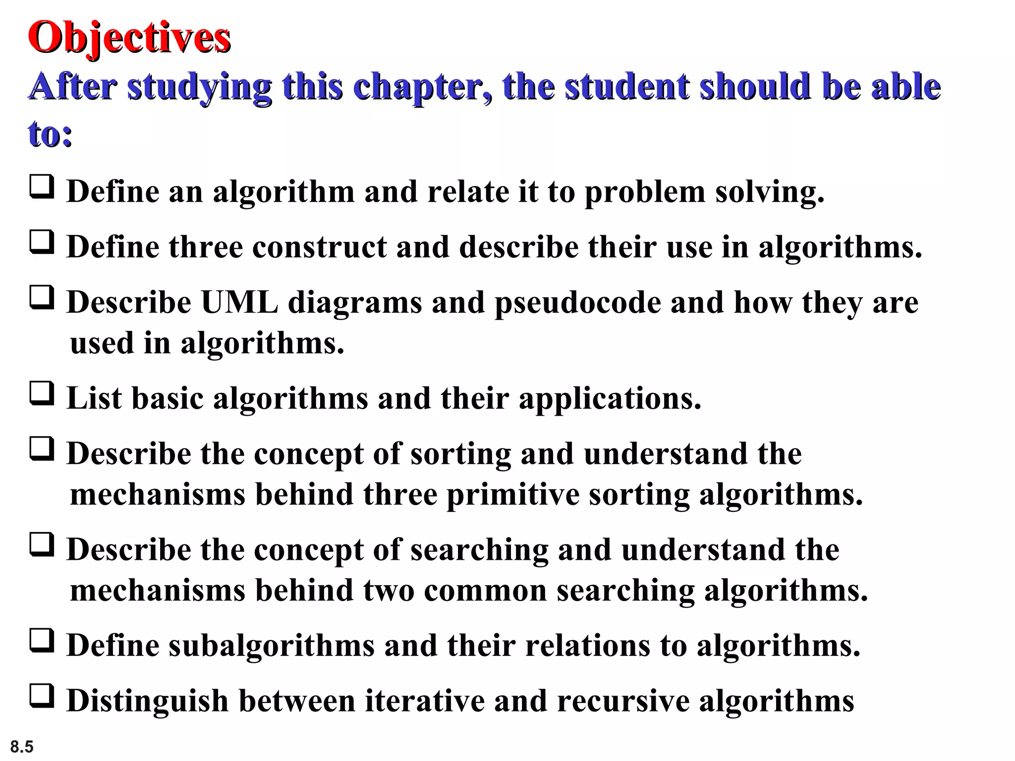
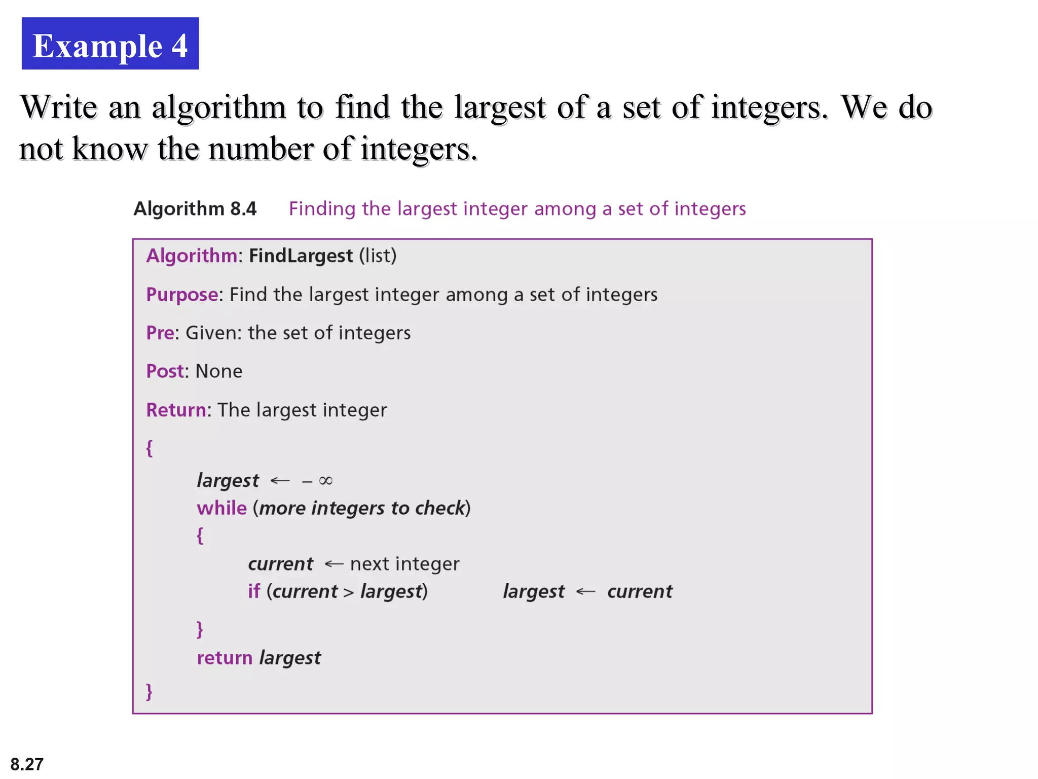
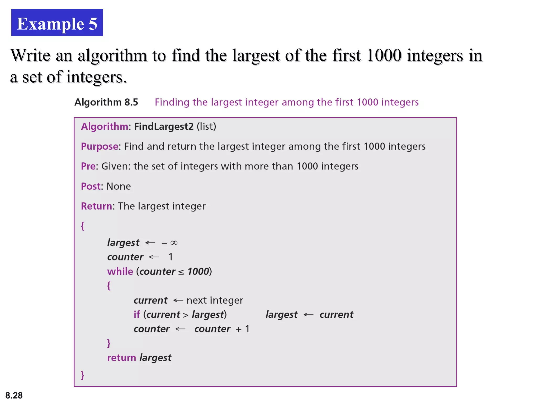
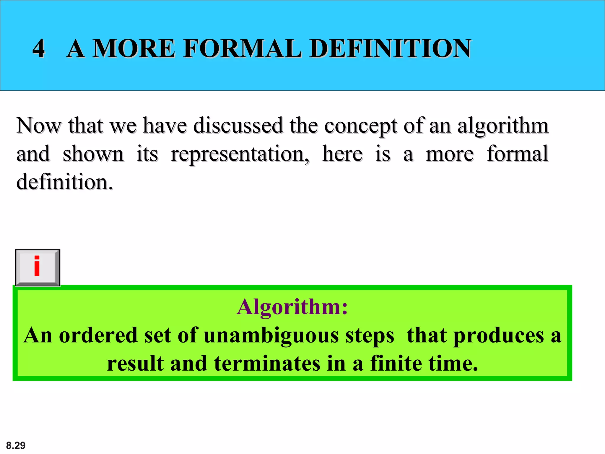
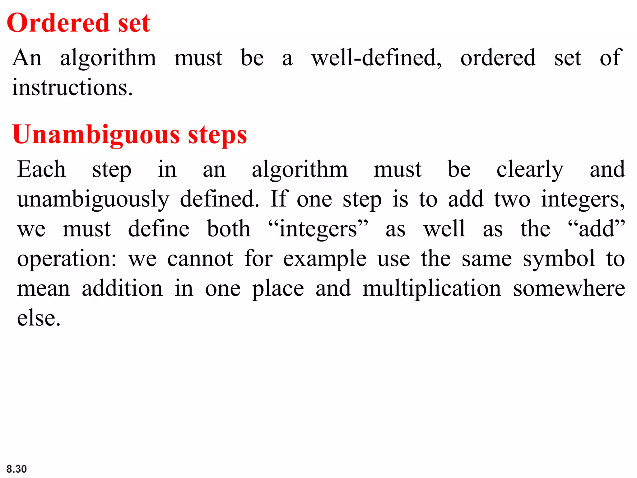
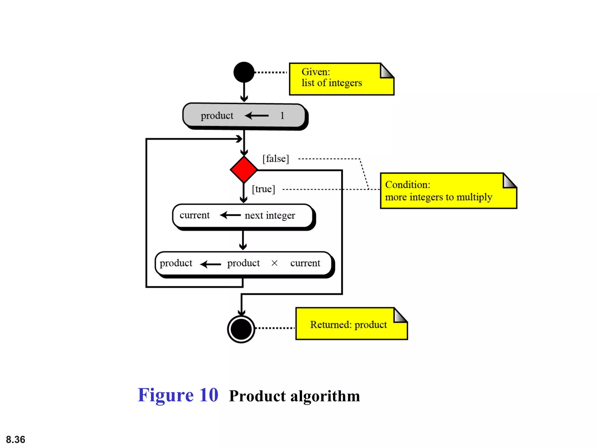
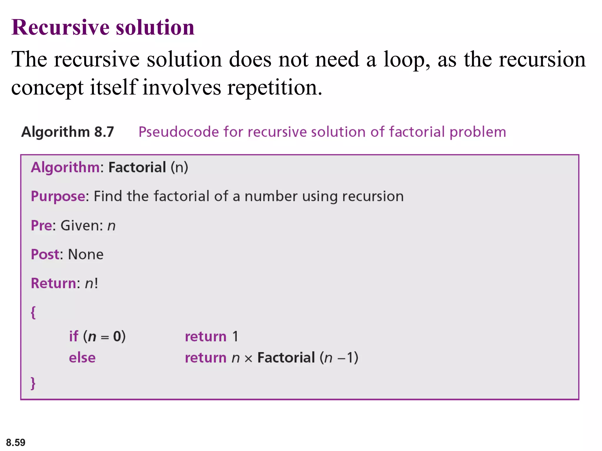
8.1
AlgorithmsAlgorithms
8.2
Algorithms for the AgesAlgorithms for the Ages
"Great algorithms are the poetry of computation""Great algorithms are the poetry of computation"
Francis SullivanFrancis Sullivan
Institute for Defense Analyses' Center for Computing SciencesInstitute for Defense Analyses' Center for Computing Sciences
Bowie, MarylandBowie, Maryland
8.3
The Importance of AlgorithmsThe Importance of Algorithms
Runtime AnalysisRuntime Analysis
8.4
The Importance of AlgorithmsThe Importance of Algorithms
SortingSorting – O(N– O(N22
))
Shortest PathShortest Path – O(C– O(CNN
) Ej: Djikstra's Algorithm) Ej: Djikstra's Algorithm
Approximate algorithmsApproximate algorithms
Random AlgorithmsRandom Algorithms – O(N– O(N22
)-O(N*log(N)) Ej: Quicksort)-O(N*log(N)) Ej: Quicksort
and medianand median
CompressionCompression
The Importance of Knowing AlgorithmsThe Importance of Knowing Algorithms
More Real-world ExamplesMore Real-world Examples
•Maximum FlowMaximum Flow
•Sequence comparisonSequence comparison
8.5
 Define an algorithm and relate it to problem solving.
 Define three construct and describe their use in algorithms.
 Describe UML diagrams and pseudocode and how they are
used in algorithms.
 List basic algorithms and their applications.
 Describe the concept of sorting and understand the
mechanisms behind three primitive sorting algorithms.
 Describe the concept of searching and understand the
mechanisms behind two common searching algorithms.
 Define subalgorithms and their relations to algorithms.
 Distinguish between iterative and recursive algorithms
ObjectivesObjectives
After studying this chapter, the student should be ableAfter studying this chapter, the student should be able
to:to:
8.6
1 CONCEPT1 CONCEPT
In this section we informally define anIn this section we informally define an algorithmalgorithm andand
elaborate on the concept using an example.elaborate on the concept using an example.
8.7
Informal definition
An informal definition of an algorithm is:
Algorithm: a step-by-step method for solving a
problem or doing a task.
Figure 1 Informal definition of an algorithm used in a computer
8.8
Example
We want to develop an algorithm for finding the largest
integer among a list of positive integers. The algorithm
should find the largest integer among a list of any values (for
example 5, 1000, 10,000, 1,000,000). The algorithm should
be general and not depend on the number of integers.
To solve this problem, we need an intuitive approach.
First use a small number of integers (for example, five), then
extend the solution to any number of integers.
Figure 2 shows one way to solve this problem. We call
the algorithm FindLargest. Each algorithm has a name to
distinguish it from other algorithms. The algorithm receives
a list of five integers as input and gives the largest integer as
output.
8.9
Figure 2 Finding the largest integer among five integers
8.10
Defining actions
Figure 2 does not show what should be done in each step.
We can modify the figure to show more details.
Figure 3 Defining actions in FindLargest algorithm
8.11
Refinement
This algorithm needs refinement to be acceptable to the
programming community. There are two problems. First, the
action in the first step is different than those for the other
steps. Second, the wording is not the same in steps 2 to 5.
We can easily redefine the algorithm to remove these two
inconveniences by changing the wording in steps 2 to 5 to
“If the current integer is greater than Largest, set Largest to
the current integer.” The reason that the first step is different
than the other steps is because Largest is not initialized. If
we initialize Largest to −∞ (minus infinity), then the first
step can be the same as the other steps, so we add a new step,
calling it step 0 to show that it should be done before
processing any integers.
8.12
Figure 4 FindLargest refined
8.13
Generalization
Is it possible to generalize the algorithm? We want to find
the largest of n positive integers, where n can be 1000,
1,000,000, or more. Of course, we can follow Figure 4 and
repeat each step. But if we change the algorithm to a
program, then we need to actually type the actions for n
steps!
There is a better way to do this. We can tell the computer to
repeat the steps n times. We now include this feature in our
pictorial algorithm (Figure 5).
8.14
Figure 5 Generalization of FindLargest
8.15
2 THREE CONSTRUCTS2 THREE CONSTRUCTS
Computer scientists have definedComputer scientists have defined three constructsthree constructs for afor a
structured program or algorithm. The idea is that astructured program or algorithm. The idea is that a
program must be made of a combination of only theseprogram must be made of a combination of only these
three constructs:three constructs: sequencesequence,, decisiondecision (selection) and(selection) and
repetitionrepetition (Figure 6). It has been proven there is no need(Figure 6). It has been proven there is no need
for any other constructs. Using only these constructsfor any other constructs. Using only these constructs
makes a program or an algorithm easy to understand,makes a program or an algorithm easy to understand,
debug or change.debug or change.
8.16
Figure 6 Three constructs
8.17
Sequence
The first construct is called the sequence. An algorithm, and
eventually a program, is a sequence of instructions, which
can be a simple instruction or either of the other two
constructs.
Decision
Some problems cannot be solved with only a sequence of
simple instructions. Sometimes we need to test a condition.
If the result of testing is true, we follow a sequence of
instructions: if it is false, we follow a different sequence of
instructions. This is called the decision (selection) construct.
8.18
Repetition
In some problems, the same sequence of instructions must be
repeated. We handle this with the repetition or loop
construct. Finding the largest integer among a set of integers
can use a construct of this kind.
8.19
3 ALGORITHM REPRESENTATION3 ALGORITHM REPRESENTATION
So far, we have used figures to convey the concept of anSo far, we have used figures to convey the concept of an
algorithm. During the last few decades, tools have beenalgorithm. During the last few decades, tools have been
designed for this purpose. Two of these tools,designed for this purpose. Two of these tools, UMLUML andand
pseudocodepseudocode, are presented here., are presented here.
8.20
UML
Unified Modeling Language (UML) is a pictorial
representation of an algorithm. It hides all the details of an
algorithm in an attempt to give the “big picture” and to show
how the algorithm flows from beginning to end. UML is
covered in detail in Appendix B. Here we show only how the
three constructs are represented using UML (Figure 7)
.
8.21
Figure 7 UML for three constructs
8.22
Pseudocode
Pseudocode is an English-language-like representation of an
algorithm. There is no standard for pseudocode—some
people use a lot of detail, others use less. Some use a code
that is close to English, while others use a syntax like the
Pascal programming language.
Pseudocode is covered in detail in many books. Here we
show only how the three constructs can be represented by
pseudocode (Figure 8).
8.23
Figure 8 Pseudocode for three constructs
8.24
Example 1
Write an algorithm in pseudocode that finds the sum of twoWrite an algorithm in pseudocode that finds the sum of two
integers.integers.
8.25
Example 2
Write an algorithm to change a numeric grade to a pass/no passWrite an algorithm to change a numeric grade to a pass/no pass
grade.grade.
8.26
Example 3
Write an algorithm to change a numeric grade (integer) to a letterWrite an algorithm to change a numeric grade (integer) to a letter
grade.grade.
8.27
Example 4
Write an algorithm to find the largest of a set of integers. We doWrite an algorithm to find the largest of a set of integers. We do
not know the number of integers.not know the number of integers.
8.28
Example 5
Write an algorithm to find the largest of the first 1000 integers inWrite an algorithm to find the largest of the first 1000 integers in
a set of integers.a set of integers.
8.29
4 A MORE FORMAL DEFINITION4 A MORE FORMAL DEFINITION
Now that we have discussed the concept of an algorithmNow that we have discussed the concept of an algorithm
and shown its representation, here is a more formaland shown its representation, here is a more formal
definition.definition.
Algorithm:
An ordered set of unambiguous steps that produces a
result and terminates in a finite time.
i
8.30
Ordered set
An algorithm must be a well-defined, ordered set of
instructions.
Unambiguous steps
Each step in an algorithm must be clearly and
unambiguously defined. If one step is to add two integers,
we must define both “integers” as well as the “add”
operation: we cannot for example use the same symbol to
mean addition in one place and multiplication somewhere
else.
8.31
Produce a result
An algorithm must produce a result, otherwise it is useless.
The result can be data returned to the calling algorithm, or
some other effect (for example, printing).
Terminate in a finite time
An algorithm must terminate (halt). If it does not (that is, it
has an infinite loop), we have not created an algorithm. In
other chapters we can discuss solvable and unsolvable
problems, and we can see that a solvable problem has a
solution in the form of an algorithm that terminates.
8.32
5 BASIC ALGORITHMS5 BASIC ALGORITHMS
Several algorithms are used in computer science soSeveral algorithms are used in computer science so
prevalently that they are considered “basic”. We discussprevalently that they are considered “basic”. We discuss
the most common here. This discussion is very general:the most common here. This discussion is very general:
implementation depends on the language.implementation depends on the language.
8.33
Summation
One commonly used algorithm in computer science is
summation. We can add two or three integers very easily,
but how can we add many integers? The solution is simple:
we use the add operator in a loop (Figure 9).
A summation algorithm has three logical parts:
1. Initialization of the sum at the beginning.
2. The loop, which in each iteration adds a new integer to the
sum.
3. Return of the result after exiting from the loop.
8.34
Figure 9 Summation algorithm
8.35
Product
Another common algorithm is finding the product of a list of
integers. The solution is simple: use the multiplication
operator in a loop (Figure 10).
A product algorithm has three logical parts:
1. Initialization of the product at the beginning.
2. The loop, which in each iteration multiplies a new integer
with the product.
3. Return of the result after exiting from the loop.
8.36
Figure 10 Product algorithm
8.37
Smallest and largest
We discussed the algorithm for finding the largest among a
list of integers at the beginning of this chapter. The idea was
to write a decision construct to find the larger of two
integers. If we put this construct in a loop, we can find the
largest of a list of integers.
Finding the smallest integer among a list of integers is
similar, with two minor differences. First, we use a decision
construct to find the smaller of two integers. Second, we
initialize with a very large integer instead of a very small
one.
8.38
Sorting
One of the most common applications in computer science is
sorting, which is the process by which data is arranged
according to its values. People are surrounded by data. If the
data was not ordered, it would take hours and hours to find a
single piece of information. Imagine the difficulty of finding
someone’s telephone number in a telephone book that is not
ordered.
In this section, we introduce three sorting algorithms:
selection sort, bubble sort and insertion sort. These three
sorting algorithms are the foundation of faster sorting
algorithms used in computer science today.
8.39
Selection sorts
In a selection sort, the list to be sorted is divided into two
sublists—sorted and unsorted—which are separated by an
imaginary wall. We find the smallest element from the
unsorted sublist and swap it with the element at the
beginning of the unsorted sublist. After each selection and
swap, the imaginary wall between the two sublists moves
one element ahead.
Figure 11 Selection sort
8.40
Figure 12 Example of selection sort
8.41
Figure 13 Selection sort algorithm
8.42
Bubble sorts
In the bubble sort method, the list to be sorted is also divided
into two sublists—sorted and unsorted. The smallest element
is bubbled up from the unsorted sublist and moved to the
sorted sublist. After the smallest element has been moved to
the sorted list, the wall moves one element ahead.
Figure 14 Bubble sort
8.43
Figure 15 Example of bubble sort
8.44
Insertion sorts
The insertion sort algorithm is one of the most common
sorting techniques, and it is often used by card players. Each
card a player picks up is inserted into the proper place in
their hand of cards to maintain a particular sequence.
Figure 16 Insertion sort
8.45
Figure 17 Example of insertion sort
8.46
Searching
Another common algorithm in computer science is
searching, which is the process of finding the location of a
target among a list of objects. In the case of a list, searching
means that given a value, we want to find the location of the
first element in the list that contains that value. There are two
basic searches for lists: sequential search and binary
search. Sequential search can be used to locate an item in
any list, whereas binary search requires the list first to be
sorted.
8.47
Sequential search
Sequential search is used if the list to be searched is not
ordered. Generally, we use this technique only for small lists,
or lists that are not searched often. In other cases, the best
approach is to first sort the list and then search it using the
binary search discussed later.
In a sequential search, we start searching for the target from
the beginning of the list. We continue until we either find the
target or reach the end of the list.
8.48
Figure 18 An example of a sequential search
8.49
Binary search
The sequential search algorithm is very slow. If we have a
list of a million elements, we must do a million comparisons
in the worst case. If the list is not sorted, this is the only
solution. If the list is sorted, however, we can use a more
efficient algorithm called binary search. Generally speaking,
programmers use a binary search when a list is large.
A binary search starts by testing the data in the
element at the middle of the list. This determines whether the
target is in the first half or the second half of the list. If it is
in the first half, there is no need to further check the second
half. If it is in the second half, there is no need to further
check the first half. In other words, we eliminate half the list
from further consideration.
8.50
Figure 19 Example of a binary search
8.51
6 SUBALGORITHMS6 SUBALGORITHMS
The three programming constructs described in SectionThe three programming constructs described in Section
2 allow us to create an algorithm for any solvable2 allow us to create an algorithm for any solvable
problem. The principles of structured programming,problem. The principles of structured programming,
however, require that an algorithm be broken into smallhowever, require that an algorithm be broken into small
units calledunits called subalgorithmssubalgorithms. Each subalgorithm is in. Each subalgorithm is in
turn divided into smaller subalgorithms. A goodturn divided into smaller subalgorithms. A good
example is the algorithm for the selection sort in Figureexample is the algorithm for the selection sort in Figure
13.13.
8.52
Figure 20 Concept of a subalgorithm
8.53
Structure chart
Another tool programmers use is the structure chart. A
structure chart is a high level design tool that shows the
relationship between algorithms and subalgorithms. It is used
mainly at the design level rather than at the programming
level.
8.54
7 RECURSION7 RECURSION
In general, there are two approaches to writingIn general, there are two approaches to writing
algorithms for solving a problem. One usesalgorithms for solving a problem. One uses iterationiteration,,
the other usesthe other uses recursionrecursion. Recursion is a process in. Recursion is a process in
which an algorithm calls itself.which an algorithm calls itself.
8.55
Iterative definition
To study a simple example, consider the calculation of a
factorial. The factorial of a integer is the product of the
integral values from 1 to the integer. The definition is
iterative (Figure 21). An algorithm is iterative whenever the
definition does not involve the algorithm itself.
Figure 21 Iterative definition of factorial
8.56
Recursive definition
An algorithm is defined recursively whenever the algorithm
appears within the definition itself. For example, the factorial
function can be defined recursively as shown in Figure 22.
Figure 22 Recursive definition of factorial
8.57
Figure 23 Tracing the recursive solution to the factorial problem
8.58
Iterative solution
This solution usually involves a loop.
8.59
Recursive solution
The recursive solution does not need a loop, as the recursion
concept itself involves repetition.
8.60
The Best of the 20th Century: Top 10 Algorithms
Algos is the Greek word for pain. Algor is Latin, to be cold.
Neither is the root for algorithm, which stems instead from
al-Khwarizmi, 9th-century Arab scholar, whose book
al-jabr wa’l muqabalah devolved into today’s high school
algebra textbooks.
Al-Khwarizmi stressed the importance of methodical procedures for
solving problems.
Were he around today, he’d no doubt be impressed by the advances
in his eponymous approach.
Some of the very best algorithms of the computer age are highlighted
in the January/February 2000 issue of Computing in Science &
Engineering, a joint publication of the American Institute of Physics
and the IEEE Computer Society.
8.61
1946: John von Neumann, Stan Ulam, and Nick Metropolis,
all at the Los Alamos Scientific Laboratory, cook up the
Metropolis algorithm, also known as the Monte Carlo method.
The Metropolis algorithm aims to obtain approximate solutions
to numerical problems with unmanageably many degrees of freedom
and to combinatorial problems of factorial size, by mimicking a
random process.
Given the digital computer’s reputation for deterministic calculation,
it’s fitting that one of its earliest applications was the generation of
random numbers.
8.62
1947: George Dantzig, at the RAND Corporation, creates the
simplex method for linear programming.
In terms of widespread application, Dantzig’s algorithm is one of the
most successful of all time: Linear programming dominates the world
of industry, where economic survival depends on the ability to optimize
within budgetary and other constraints. (Of course, the “real” problems
of industry are often nonlinear; the use of linear programming is
sometimes dictated by the computational budget.)
The simplex method is an elegant way of arriving at optimal answers.
Although theoretically susceptible to exponential delays, the algorithm
in practice is highly efficient—which in itself says something interesting
about the nature of computation.
8.63
1950: Magnus Hestenes, Eduard Stiefel, and Cornelius Lanczos, from
Institute for Numerical Analysis at the National Bureau of Standards,
initiate the development of Krylov subspace iteration methods.
These algorithms address the seemingly simple task of solving equations of
form Ax = b. The catch, of course, is that A is a huge n x n matrix, so that the
algebraic answer x = b/A is not so easy to compute. (Indeed, matrix “division”
is not a particularly useful concept.) Iterative methods—such as solving
equations of the form Kxi + 1
= Kxi
+ b – Axi
with a simpler matrix K that’s
ideally “close” to A—lead to the study of Krylov subspaces. Named for the
Russian mathematician Nikolai Krylov, Krylov subspaces are spanned by
powers of a matrix applied to an initial “remainder” vector r0
= b – Ax0
.
Lanczos found a nifty way to generate an orthogonal basis for such a subspace
when the matrix is symmetric. Hestenes and Stiefel proposed an even niftier
method known as the conjugate gradient method, for systems that are both
symmetric and positive definite.
8.64
1951: Alston Householder of Oak Ridge National Laboratory
formalizes the decompositional approach to matrix computations
The ability to factor matrices into triangular, diagonal, orthogonal,
and other special forms has turned out to be extremely useful. The
decompositional approach has enabled software developers to produce
flexible and efficient matrix packages. It also facilitates the analysis of
rounding errors, one of the big bugbears of numerical linear algebra.
In 1961, James Wilkinson of the National Physical Laboratory in
London published a seminal paper in the Journal of the ACM, titled
“Error Analysis of Direct Methods of Matrix Inversion”, based on the
LU decomposition of a matrix as a product of Lower and Upper
triangular factors.
8.65
1957: John Backus leads a team at IBM in developing the
Fortran optimizing compiler.
The creation of Fortran may rank as the single most important event
in the history of computer programming: Finally, scientists (and others)
could tell the computer what they wanted it to do, without having to
descend into the netherworld of machine code.
Although modest by modern compiler standards—Fortran I consisted
of a mere 23,500 assembly-language instructions—the early compiler
was nonetheless capable of surprisingly sophisticated computations.
As Backus himself recalls in a recent history of Fortran I, II, and III,
published in 1998 in the IEEE Annals of the History of Computing, the
compiler “produced code of such efficiency that its output would startle
the programmers who studied it.”
8.66
1959–61: J.G.F. Francis of Ferranti Ltd., London, finds a stable
method for computing eigenvalues, known as the QR algorithm.
Eigenvalues are arguably the most important numbers associated with
matrices—and they can be the trickiest to compute. It’s relatively easy
to transform a square matrix into a matrix that’s “almost” upper
triangular, meaning one with a single extra set of nonzero entries just
below the main diagonal.
But chipping away those final nonzeros, without launching an
avalanche of error, is nontrivial. The QR algorithm is just the ticket.
Based on the QR decomposition, which writes A as the product of an
orthogonal matrix Q and an upper triangular matrix R, this approach
iteratively changes Ai
= QR into Ai + 1
= RQ, with a few bells and
whistles for accelerating convergence to upper triangular form.
By the mid-1960s, the QR algorithm had turned once-formidable
eigenvalue problems into routine calculations.
8.67
1962: Tony Hoare of Elliott Brothers, Ltd., London, presents
Quicksort.
Putting N things in numerical or alphabetical order is mind-
numbingly mundane. The intellectual challenge lies in devising ways
of doing so quickly.
Hoare’s algorithm uses the age-old recursive strategy of divide and
conquer to solve the problem: Pick one element as a “pivot,” separate
the rest into piles of “big” and “small” elements (as compared with
the pivot), and then repeat this procedure on each pile. Although it’s
possible to get stuck doing all N(N – 1)/2 comparisons (especially if
you use as your pivot the first item on a list that’s already sorted!),
Quicksort runs on average with O(N log N) efficiency. Its elegant
simplicity has made Quicksort the posterchild of computational
complexity.
8.68
1965: James Cooley of the IBM T.J. Watson Research Center and
John Tukey of Princeton University and AT&T Bell Laboratories
unveil the Fast Fourier Transform.
Easily the most far-reaching algorithm in applied mathematics, the FFT
revolutionized signal processing. The underlying idea goes back to Gauss
(who needed to calculate orbits of asteroids), but it was the Cooley–Tukey
paper that made it clear how easily Fourier transforms can be computed.
Like Quicksort, the FFT relies on a divide-and-conquer strategy to reduce
an ostensibly O(N2
) chore to an O(N log N) frolic. But unlike Quicksort,
the implementation is (at first sight) nonintuitive and less than straight
forward.
This in itself gave computer science an impetus to investigate the inherent
complexity of computational problems and algorithms.
8.69
1977: Helaman Ferguson and Rodney Forcade of Brigham Young
University advance an integer relation detection algorithm
The problem is an old one: Given a bunch of real numbers, say
x1
, x2
, . . . , xn
, are there integers a1
, a2
, . . . , an
(not all 0) for which
a1
x1
+ a2
x2
+ . . . + an
xn
= 0? For n = 2, the venerable Euclidean
algorithm does the job, computing terms in the continued-fraction
expansion of x1
/x2
. If x1
/x2
is rational, the expansion terminates and,
with proper unraveling, gives the “smallest” integers a1
and a2
. If the
Euclidean algorithm doesn’t terminate—or if you simply get tired
of computing it—then the unraveling procedure at least provides lower
bounds on the size of the smallest integer relation.
Ferguson and Forcade’s generalization, although much more difficult
to implement (and to understand), is also more powerful. Their detection
algorithm, for example, has been used to find the precise coefficients of
the polynomials satisfied by the third and fourth bifurcation points,
B3 = 3.544090 and B4 = 3.564407, of the logistic map. (The latter
polynomial is of degree 120; its largest coefficient is 25730.) It has also
proved useful in simplifying calculations with Feynman diagrams in QFT.
8.70
1987: Leslie Greengard and Vladimir Rokhlin of Yale University
invent the fast multipole algorithm.
This algorithm overcomes one of the biggest headaches of N-body
simulations: the fact that accurate calculations of the motions
of N particles interacting via gravitational or electrostatic forces
(think stars in a galaxy, or atoms in a protein) would seem to require
O(N2
) computations—one for each pair of particles. The fast
multipole algorithm gets by with O(N) computations. It does so by
using multipole expansions (net charge or mass, dipole moment,
quadrupole, and so forth) to approximate the effects of a distant
group of particles on a local group. A hierarchical decomposition of
space is used to define ever-larger groups as distances increase.
One of the distinct advantages of the fast multipole algorithm is that
it comes equipped with rigorous error estimates, a feature that
many methods lack.

Algoritmos

  • 1.
  • 2.
    8.2 Algorithms for theAgesAlgorithms for the Ages "Great algorithms are the poetry of computation""Great algorithms are the poetry of computation" Francis SullivanFrancis Sullivan Institute for Defense Analyses' Center for Computing SciencesInstitute for Defense Analyses' Center for Computing Sciences Bowie, MarylandBowie, Maryland
  • 3.
    8.3 The Importance ofAlgorithmsThe Importance of Algorithms Runtime AnalysisRuntime Analysis
  • 4.
    8.4 The Importance ofAlgorithmsThe Importance of Algorithms SortingSorting – O(N– O(N22 )) Shortest PathShortest Path – O(C– O(CNN ) Ej: Djikstra's Algorithm) Ej: Djikstra's Algorithm Approximate algorithmsApproximate algorithms Random AlgorithmsRandom Algorithms – O(N– O(N22 )-O(N*log(N)) Ej: Quicksort)-O(N*log(N)) Ej: Quicksort and medianand median CompressionCompression The Importance of Knowing AlgorithmsThe Importance of Knowing Algorithms More Real-world ExamplesMore Real-world Examples •Maximum FlowMaximum Flow •Sequence comparisonSequence comparison
  • 5.
    8.5  Define analgorithm and relate it to problem solving.  Define three construct and describe their use in algorithms.  Describe UML diagrams and pseudocode and how they are used in algorithms.  List basic algorithms and their applications.  Describe the concept of sorting and understand the mechanisms behind three primitive sorting algorithms.  Describe the concept of searching and understand the mechanisms behind two common searching algorithms.  Define subalgorithms and their relations to algorithms.  Distinguish between iterative and recursive algorithms ObjectivesObjectives After studying this chapter, the student should be ableAfter studying this chapter, the student should be able to:to:
  • 6.
    8.6 1 CONCEPT1 CONCEPT Inthis section we informally define anIn this section we informally define an algorithmalgorithm andand elaborate on the concept using an example.elaborate on the concept using an example.
  • 7.
    8.7 Informal definition An informaldefinition of an algorithm is: Algorithm: a step-by-step method for solving a problem or doing a task. Figure 1 Informal definition of an algorithm used in a computer
  • 8.
    8.8 Example We want todevelop an algorithm for finding the largest integer among a list of positive integers. The algorithm should find the largest integer among a list of any values (for example 5, 1000, 10,000, 1,000,000). The algorithm should be general and not depend on the number of integers. To solve this problem, we need an intuitive approach. First use a small number of integers (for example, five), then extend the solution to any number of integers. Figure 2 shows one way to solve this problem. We call the algorithm FindLargest. Each algorithm has a name to distinguish it from other algorithms. The algorithm receives a list of five integers as input and gives the largest integer as output.
  • 9.
    8.9 Figure 2 Findingthe largest integer among five integers
  • 10.
    8.10 Defining actions Figure 2does not show what should be done in each step. We can modify the figure to show more details. Figure 3 Defining actions in FindLargest algorithm
  • 11.
    8.11 Refinement This algorithm needsrefinement to be acceptable to the programming community. There are two problems. First, the action in the first step is different than those for the other steps. Second, the wording is not the same in steps 2 to 5. We can easily redefine the algorithm to remove these two inconveniences by changing the wording in steps 2 to 5 to “If the current integer is greater than Largest, set Largest to the current integer.” The reason that the first step is different than the other steps is because Largest is not initialized. If we initialize Largest to −∞ (minus infinity), then the first step can be the same as the other steps, so we add a new step, calling it step 0 to show that it should be done before processing any integers.
  • 12.
  • 13.
    8.13 Generalization Is it possibleto generalize the algorithm? We want to find the largest of n positive integers, where n can be 1000, 1,000,000, or more. Of course, we can follow Figure 4 and repeat each step. But if we change the algorithm to a program, then we need to actually type the actions for n steps! There is a better way to do this. We can tell the computer to repeat the steps n times. We now include this feature in our pictorial algorithm (Figure 5).
  • 14.
  • 15.
    8.15 2 THREE CONSTRUCTS2THREE CONSTRUCTS Computer scientists have definedComputer scientists have defined three constructsthree constructs for afor a structured program or algorithm. The idea is that astructured program or algorithm. The idea is that a program must be made of a combination of only theseprogram must be made of a combination of only these three constructs:three constructs: sequencesequence,, decisiondecision (selection) and(selection) and repetitionrepetition (Figure 6). It has been proven there is no need(Figure 6). It has been proven there is no need for any other constructs. Using only these constructsfor any other constructs. Using only these constructs makes a program or an algorithm easy to understand,makes a program or an algorithm easy to understand, debug or change.debug or change.
  • 16.
  • 17.
    8.17 Sequence The first constructis called the sequence. An algorithm, and eventually a program, is a sequence of instructions, which can be a simple instruction or either of the other two constructs. Decision Some problems cannot be solved with only a sequence of simple instructions. Sometimes we need to test a condition. If the result of testing is true, we follow a sequence of instructions: if it is false, we follow a different sequence of instructions. This is called the decision (selection) construct.
  • 18.
    8.18 Repetition In some problems,the same sequence of instructions must be repeated. We handle this with the repetition or loop construct. Finding the largest integer among a set of integers can use a construct of this kind.
  • 19.
    8.19 3 ALGORITHM REPRESENTATION3ALGORITHM REPRESENTATION So far, we have used figures to convey the concept of anSo far, we have used figures to convey the concept of an algorithm. During the last few decades, tools have beenalgorithm. During the last few decades, tools have been designed for this purpose. Two of these tools,designed for this purpose. Two of these tools, UMLUML andand pseudocodepseudocode, are presented here., are presented here.
  • 20.
    8.20 UML Unified Modeling Language(UML) is a pictorial representation of an algorithm. It hides all the details of an algorithm in an attempt to give the “big picture” and to show how the algorithm flows from beginning to end. UML is covered in detail in Appendix B. Here we show only how the three constructs are represented using UML (Figure 7) .
  • 21.
    8.21 Figure 7 UMLfor three constructs
  • 22.
    8.22 Pseudocode Pseudocode is anEnglish-language-like representation of an algorithm. There is no standard for pseudocode—some people use a lot of detail, others use less. Some use a code that is close to English, while others use a syntax like the Pascal programming language. Pseudocode is covered in detail in many books. Here we show only how the three constructs can be represented by pseudocode (Figure 8).
  • 23.
    8.23 Figure 8 Pseudocodefor three constructs
  • 24.
    8.24 Example 1 Write analgorithm in pseudocode that finds the sum of twoWrite an algorithm in pseudocode that finds the sum of two integers.integers.
  • 25.
    8.25 Example 2 Write analgorithm to change a numeric grade to a pass/no passWrite an algorithm to change a numeric grade to a pass/no pass grade.grade.
  • 26.
    8.26 Example 3 Write analgorithm to change a numeric grade (integer) to a letterWrite an algorithm to change a numeric grade (integer) to a letter grade.grade.
  • 27.
    8.27 Example 4 Write analgorithm to find the largest of a set of integers. We doWrite an algorithm to find the largest of a set of integers. We do not know the number of integers.not know the number of integers.
  • 28.
    8.28 Example 5 Write analgorithm to find the largest of the first 1000 integers inWrite an algorithm to find the largest of the first 1000 integers in a set of integers.a set of integers.
  • 29.
    8.29 4 A MOREFORMAL DEFINITION4 A MORE FORMAL DEFINITION Now that we have discussed the concept of an algorithmNow that we have discussed the concept of an algorithm and shown its representation, here is a more formaland shown its representation, here is a more formal definition.definition. Algorithm: An ordered set of unambiguous steps that produces a result and terminates in a finite time. i
  • 30.
    8.30 Ordered set An algorithmmust be a well-defined, ordered set of instructions. Unambiguous steps Each step in an algorithm must be clearly and unambiguously defined. If one step is to add two integers, we must define both “integers” as well as the “add” operation: we cannot for example use the same symbol to mean addition in one place and multiplication somewhere else.
  • 31.
    8.31 Produce a result Analgorithm must produce a result, otherwise it is useless. The result can be data returned to the calling algorithm, or some other effect (for example, printing). Terminate in a finite time An algorithm must terminate (halt). If it does not (that is, it has an infinite loop), we have not created an algorithm. In other chapters we can discuss solvable and unsolvable problems, and we can see that a solvable problem has a solution in the form of an algorithm that terminates.
  • 32.
    8.32 5 BASIC ALGORITHMS5BASIC ALGORITHMS Several algorithms are used in computer science soSeveral algorithms are used in computer science so prevalently that they are considered “basic”. We discussprevalently that they are considered “basic”. We discuss the most common here. This discussion is very general:the most common here. This discussion is very general: implementation depends on the language.implementation depends on the language.
  • 33.
    8.33 Summation One commonly usedalgorithm in computer science is summation. We can add two or three integers very easily, but how can we add many integers? The solution is simple: we use the add operator in a loop (Figure 9). A summation algorithm has three logical parts: 1. Initialization of the sum at the beginning. 2. The loop, which in each iteration adds a new integer to the sum. 3. Return of the result after exiting from the loop.
  • 34.
  • 35.
    8.35 Product Another common algorithmis finding the product of a list of integers. The solution is simple: use the multiplication operator in a loop (Figure 10). A product algorithm has three logical parts: 1. Initialization of the product at the beginning. 2. The loop, which in each iteration multiplies a new integer with the product. 3. Return of the result after exiting from the loop.
  • 36.
  • 37.
    8.37 Smallest and largest Wediscussed the algorithm for finding the largest among a list of integers at the beginning of this chapter. The idea was to write a decision construct to find the larger of two integers. If we put this construct in a loop, we can find the largest of a list of integers. Finding the smallest integer among a list of integers is similar, with two minor differences. First, we use a decision construct to find the smaller of two integers. Second, we initialize with a very large integer instead of a very small one.
  • 38.
    8.38 Sorting One of themost common applications in computer science is sorting, which is the process by which data is arranged according to its values. People are surrounded by data. If the data was not ordered, it would take hours and hours to find a single piece of information. Imagine the difficulty of finding someone’s telephone number in a telephone book that is not ordered. In this section, we introduce three sorting algorithms: selection sort, bubble sort and insertion sort. These three sorting algorithms are the foundation of faster sorting algorithms used in computer science today.
  • 39.
    8.39 Selection sorts In aselection sort, the list to be sorted is divided into two sublists—sorted and unsorted—which are separated by an imaginary wall. We find the smallest element from the unsorted sublist and swap it with the element at the beginning of the unsorted sublist. After each selection and swap, the imaginary wall between the two sublists moves one element ahead. Figure 11 Selection sort
  • 40.
    8.40 Figure 12 Exampleof selection sort
  • 41.
  • 42.
    8.42 Bubble sorts In thebubble sort method, the list to be sorted is also divided into two sublists—sorted and unsorted. The smallest element is bubbled up from the unsorted sublist and moved to the sorted sublist. After the smallest element has been moved to the sorted list, the wall moves one element ahead. Figure 14 Bubble sort
  • 43.
    8.43 Figure 15 Exampleof bubble sort
  • 44.
    8.44 Insertion sorts The insertionsort algorithm is one of the most common sorting techniques, and it is often used by card players. Each card a player picks up is inserted into the proper place in their hand of cards to maintain a particular sequence. Figure 16 Insertion sort
  • 45.
    8.45 Figure 17 Exampleof insertion sort
  • 46.
    8.46 Searching Another common algorithmin computer science is searching, which is the process of finding the location of a target among a list of objects. In the case of a list, searching means that given a value, we want to find the location of the first element in the list that contains that value. There are two basic searches for lists: sequential search and binary search. Sequential search can be used to locate an item in any list, whereas binary search requires the list first to be sorted.
  • 47.
    8.47 Sequential search Sequential searchis used if the list to be searched is not ordered. Generally, we use this technique only for small lists, or lists that are not searched often. In other cases, the best approach is to first sort the list and then search it using the binary search discussed later. In a sequential search, we start searching for the target from the beginning of the list. We continue until we either find the target or reach the end of the list.
  • 48.
    8.48 Figure 18 Anexample of a sequential search
  • 49.
    8.49 Binary search The sequentialsearch algorithm is very slow. If we have a list of a million elements, we must do a million comparisons in the worst case. If the list is not sorted, this is the only solution. If the list is sorted, however, we can use a more efficient algorithm called binary search. Generally speaking, programmers use a binary search when a list is large. A binary search starts by testing the data in the element at the middle of the list. This determines whether the target is in the first half or the second half of the list. If it is in the first half, there is no need to further check the second half. If it is in the second half, there is no need to further check the first half. In other words, we eliminate half the list from further consideration.
  • 50.
    8.50 Figure 19 Exampleof a binary search
  • 51.
    8.51 6 SUBALGORITHMS6 SUBALGORITHMS Thethree programming constructs described in SectionThe three programming constructs described in Section 2 allow us to create an algorithm for any solvable2 allow us to create an algorithm for any solvable problem. The principles of structured programming,problem. The principles of structured programming, however, require that an algorithm be broken into smallhowever, require that an algorithm be broken into small units calledunits called subalgorithmssubalgorithms. Each subalgorithm is in. Each subalgorithm is in turn divided into smaller subalgorithms. A goodturn divided into smaller subalgorithms. A good example is the algorithm for the selection sort in Figureexample is the algorithm for the selection sort in Figure 13.13.
  • 52.
    8.52 Figure 20 Conceptof a subalgorithm
  • 53.
    8.53 Structure chart Another toolprogrammers use is the structure chart. A structure chart is a high level design tool that shows the relationship between algorithms and subalgorithms. It is used mainly at the design level rather than at the programming level.
  • 54.
    8.54 7 RECURSION7 RECURSION Ingeneral, there are two approaches to writingIn general, there are two approaches to writing algorithms for solving a problem. One usesalgorithms for solving a problem. One uses iterationiteration,, the other usesthe other uses recursionrecursion. Recursion is a process in. Recursion is a process in which an algorithm calls itself.which an algorithm calls itself.
  • 55.
    8.55 Iterative definition To studya simple example, consider the calculation of a factorial. The factorial of a integer is the product of the integral values from 1 to the integer. The definition is iterative (Figure 21). An algorithm is iterative whenever the definition does not involve the algorithm itself. Figure 21 Iterative definition of factorial
  • 56.
    8.56 Recursive definition An algorithmis defined recursively whenever the algorithm appears within the definition itself. For example, the factorial function can be defined recursively as shown in Figure 22. Figure 22 Recursive definition of factorial
  • 57.
    8.57 Figure 23 Tracingthe recursive solution to the factorial problem
  • 58.
    8.58 Iterative solution This solutionusually involves a loop.
  • 59.
    8.59 Recursive solution The recursivesolution does not need a loop, as the recursion concept itself involves repetition.
  • 60.
    8.60 The Best ofthe 20th Century: Top 10 Algorithms Algos is the Greek word for pain. Algor is Latin, to be cold. Neither is the root for algorithm, which stems instead from al-Khwarizmi, 9th-century Arab scholar, whose book al-jabr wa’l muqabalah devolved into today’s high school algebra textbooks. Al-Khwarizmi stressed the importance of methodical procedures for solving problems. Were he around today, he’d no doubt be impressed by the advances in his eponymous approach. Some of the very best algorithms of the computer age are highlighted in the January/February 2000 issue of Computing in Science & Engineering, a joint publication of the American Institute of Physics and the IEEE Computer Society.
  • 61.
    8.61 1946: John vonNeumann, Stan Ulam, and Nick Metropolis, all at the Los Alamos Scientific Laboratory, cook up the Metropolis algorithm, also known as the Monte Carlo method. The Metropolis algorithm aims to obtain approximate solutions to numerical problems with unmanageably many degrees of freedom and to combinatorial problems of factorial size, by mimicking a random process. Given the digital computer’s reputation for deterministic calculation, it’s fitting that one of its earliest applications was the generation of random numbers.
  • 62.
    8.62 1947: George Dantzig,at the RAND Corporation, creates the simplex method for linear programming. In terms of widespread application, Dantzig’s algorithm is one of the most successful of all time: Linear programming dominates the world of industry, where economic survival depends on the ability to optimize within budgetary and other constraints. (Of course, the “real” problems of industry are often nonlinear; the use of linear programming is sometimes dictated by the computational budget.) The simplex method is an elegant way of arriving at optimal answers. Although theoretically susceptible to exponential delays, the algorithm in practice is highly efficient—which in itself says something interesting about the nature of computation.
  • 63.
    8.63 1950: Magnus Hestenes,Eduard Stiefel, and Cornelius Lanczos, from Institute for Numerical Analysis at the National Bureau of Standards, initiate the development of Krylov subspace iteration methods. These algorithms address the seemingly simple task of solving equations of form Ax = b. The catch, of course, is that A is a huge n x n matrix, so that the algebraic answer x = b/A is not so easy to compute. (Indeed, matrix “division” is not a particularly useful concept.) Iterative methods—such as solving equations of the form Kxi + 1 = Kxi + b – Axi with a simpler matrix K that’s ideally “close” to A—lead to the study of Krylov subspaces. Named for the Russian mathematician Nikolai Krylov, Krylov subspaces are spanned by powers of a matrix applied to an initial “remainder” vector r0 = b – Ax0 . Lanczos found a nifty way to generate an orthogonal basis for such a subspace when the matrix is symmetric. Hestenes and Stiefel proposed an even niftier method known as the conjugate gradient method, for systems that are both symmetric and positive definite.
  • 64.
    8.64 1951: Alston Householderof Oak Ridge National Laboratory formalizes the decompositional approach to matrix computations The ability to factor matrices into triangular, diagonal, orthogonal, and other special forms has turned out to be extremely useful. The decompositional approach has enabled software developers to produce flexible and efficient matrix packages. It also facilitates the analysis of rounding errors, one of the big bugbears of numerical linear algebra. In 1961, James Wilkinson of the National Physical Laboratory in London published a seminal paper in the Journal of the ACM, titled “Error Analysis of Direct Methods of Matrix Inversion”, based on the LU decomposition of a matrix as a product of Lower and Upper triangular factors.
  • 65.
    8.65 1957: John Backusleads a team at IBM in developing the Fortran optimizing compiler. The creation of Fortran may rank as the single most important event in the history of computer programming: Finally, scientists (and others) could tell the computer what they wanted it to do, without having to descend into the netherworld of machine code. Although modest by modern compiler standards—Fortran I consisted of a mere 23,500 assembly-language instructions—the early compiler was nonetheless capable of surprisingly sophisticated computations. As Backus himself recalls in a recent history of Fortran I, II, and III, published in 1998 in the IEEE Annals of the History of Computing, the compiler “produced code of such efficiency that its output would startle the programmers who studied it.”
  • 66.
    8.66 1959–61: J.G.F. Francisof Ferranti Ltd., London, finds a stable method for computing eigenvalues, known as the QR algorithm. Eigenvalues are arguably the most important numbers associated with matrices—and they can be the trickiest to compute. It’s relatively easy to transform a square matrix into a matrix that’s “almost” upper triangular, meaning one with a single extra set of nonzero entries just below the main diagonal. But chipping away those final nonzeros, without launching an avalanche of error, is nontrivial. The QR algorithm is just the ticket. Based on the QR decomposition, which writes A as the product of an orthogonal matrix Q and an upper triangular matrix R, this approach iteratively changes Ai = QR into Ai + 1 = RQ, with a few bells and whistles for accelerating convergence to upper triangular form. By the mid-1960s, the QR algorithm had turned once-formidable eigenvalue problems into routine calculations.
  • 67.
    8.67 1962: Tony Hoareof Elliott Brothers, Ltd., London, presents Quicksort. Putting N things in numerical or alphabetical order is mind- numbingly mundane. The intellectual challenge lies in devising ways of doing so quickly. Hoare’s algorithm uses the age-old recursive strategy of divide and conquer to solve the problem: Pick one element as a “pivot,” separate the rest into piles of “big” and “small” elements (as compared with the pivot), and then repeat this procedure on each pile. Although it’s possible to get stuck doing all N(N – 1)/2 comparisons (especially if you use as your pivot the first item on a list that’s already sorted!), Quicksort runs on average with O(N log N) efficiency. Its elegant simplicity has made Quicksort the posterchild of computational complexity.
  • 68.
    8.68 1965: James Cooleyof the IBM T.J. Watson Research Center and John Tukey of Princeton University and AT&T Bell Laboratories unveil the Fast Fourier Transform. Easily the most far-reaching algorithm in applied mathematics, the FFT revolutionized signal processing. The underlying idea goes back to Gauss (who needed to calculate orbits of asteroids), but it was the Cooley–Tukey paper that made it clear how easily Fourier transforms can be computed. Like Quicksort, the FFT relies on a divide-and-conquer strategy to reduce an ostensibly O(N2 ) chore to an O(N log N) frolic. But unlike Quicksort, the implementation is (at first sight) nonintuitive and less than straight forward. This in itself gave computer science an impetus to investigate the inherent complexity of computational problems and algorithms.
  • 69.
    8.69 1977: Helaman Fergusonand Rodney Forcade of Brigham Young University advance an integer relation detection algorithm The problem is an old one: Given a bunch of real numbers, say x1 , x2 , . . . , xn , are there integers a1 , a2 , . . . , an (not all 0) for which a1 x1 + a2 x2 + . . . + an xn = 0? For n = 2, the venerable Euclidean algorithm does the job, computing terms in the continued-fraction expansion of x1 /x2 . If x1 /x2 is rational, the expansion terminates and, with proper unraveling, gives the “smallest” integers a1 and a2 . If the Euclidean algorithm doesn’t terminate—or if you simply get tired of computing it—then the unraveling procedure at least provides lower bounds on the size of the smallest integer relation. Ferguson and Forcade’s generalization, although much more difficult to implement (and to understand), is also more powerful. Their detection algorithm, for example, has been used to find the precise coefficients of the polynomials satisfied by the third and fourth bifurcation points, B3 = 3.544090 and B4 = 3.564407, of the logistic map. (The latter polynomial is of degree 120; its largest coefficient is 25730.) It has also proved useful in simplifying calculations with Feynman diagrams in QFT.
  • 70.
    8.70 1987: Leslie Greengardand Vladimir Rokhlin of Yale University invent the fast multipole algorithm. This algorithm overcomes one of the biggest headaches of N-body simulations: the fact that accurate calculations of the motions of N particles interacting via gravitational or electrostatic forces (think stars in a galaxy, or atoms in a protein) would seem to require O(N2 ) computations—one for each pair of particles. The fast multipole algorithm gets by with O(N) computations. It does so by using multipole expansions (net charge or mass, dipole moment, quadrupole, and so forth) to approximate the effects of a distant group of particles on a local group. A hierarchical decomposition of space is used to define ever-larger groups as distances increase. One of the distinct advantages of the fast multipole algorithm is that it comes equipped with rigorous error estimates, a feature that many methods lack.