Download as PDF, PPTX


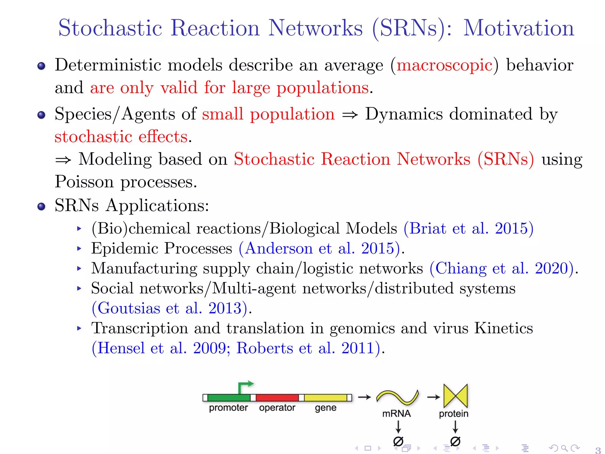
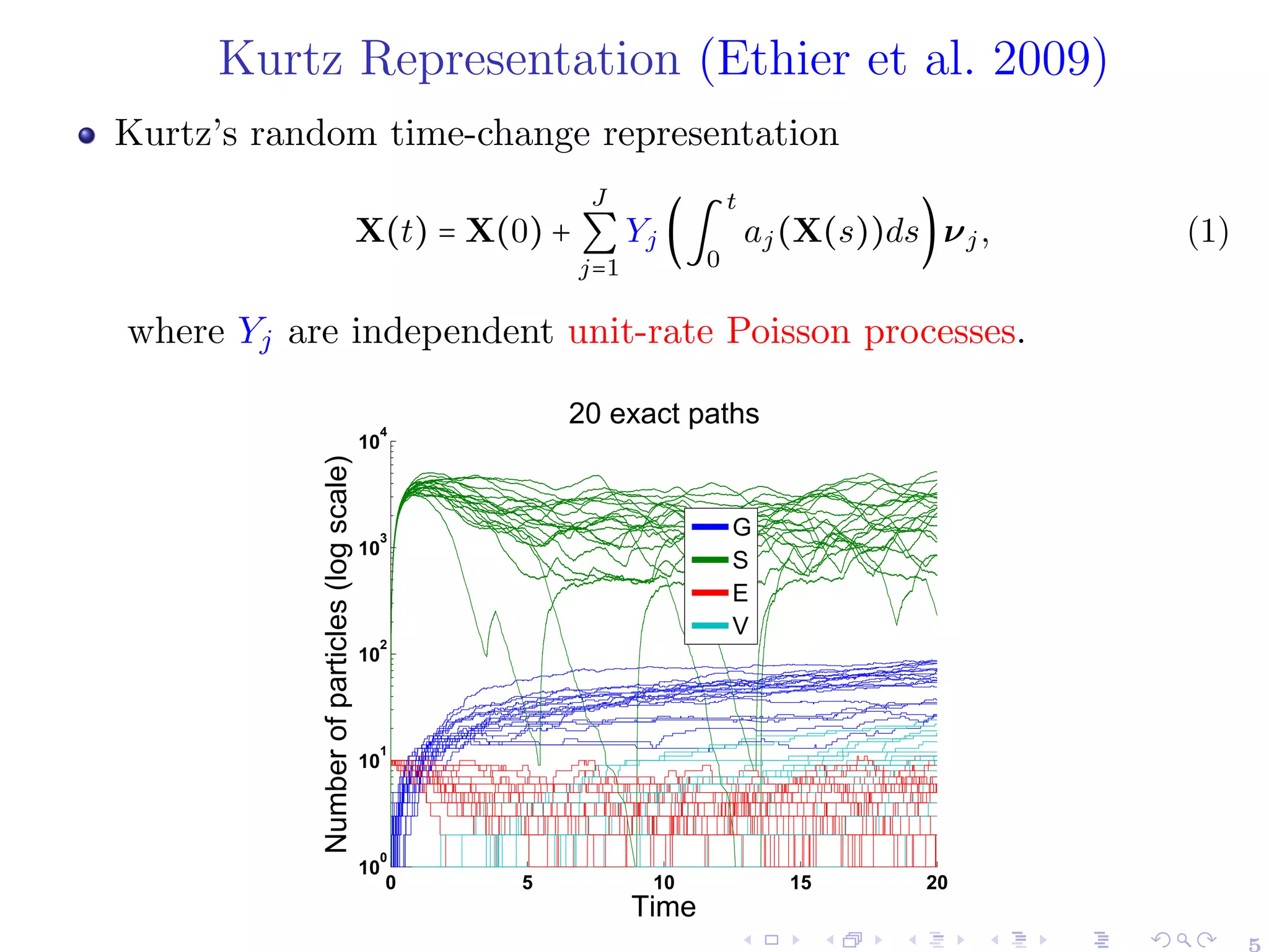
![Stochastic Reaction Network (SRNs)
A stochastic reaction network (SRN) is a continuous-time Markov
chain, X(t), defined on a probability space (Ω,F,P)1
X(t) = (X(1)
(t),...,X(d)
(t)) ∶ [0,T] × Ω → Nd
described by J reactions channels, Rj ∶= (νj,aj), where
▸ νj ∈ Zd
: stoichiometric (state change) vector.
▸ aj ∶ Rd
+ → R+: propensity (jump intensity) function.
aj satisfies
P(X(t + ∆t) = x + νj ∣ X(t) = x) = aj(x)∆t + o(∆t), j = 1,...,J.
1
X(i)
(t) may describe the abundance (counting number) of the i-th species
(agent) present in the system at time t. 4](https://image.slidesharecdn.com/kausttalkshort-230531154446-ae89ff73/75/KAUST_talk_short-pdf-6-2048.jpg)
![Importance Sampling (IS) for MC
Let Y be a real r.v.
IS is a change of measure, and it reduces the MC computational
cost by sampling on regions with the most effect on the QoI.
Instead of approximating EP
[Y ] with MC, IS uses MC for
EQ
[Y dP
dQ ].
The minimum variance is then
V arQ∗
[Y
dP
dQ∗
] = (EP
[∣Y ∣])
2
(1 − (EQ∗
[1{Y >0}] − EQ∗
[1{Y <0}])
2
)
IS-MC will be more efficient than plain MC when
V arP
[Y ]/(EP
[∣Y ∣])
2
>> 1 or Y has near constant sign, i.e.
V arQ∗
[Y
dP
dQ∗
](1 + θ) < V arP
[Y ]
Here (1 + θ) ≥ 1 is the relative cost of sampling Y dP
dQ∗ under Q∗
wrt sampling Y under P.
8](https://image.slidesharecdn.com/kausttalkshort-230531154446-ae89ff73/75/KAUST_talk_short-pdf-10-2048.jpg)
![Aim and Setting
Design a computationally efficient MC estimator for
E[g(X(T))] using IS:
▸ We are interested in g(X(T)) = 1{X(T )∈B} for a set B ⊆ Nd
for
rare event applications: E[g(X(T))] = P(X(T) ∈ B) ≪ 1
▸ {X(t) ∶ t ∈ [0,T]} is a SRNs.
Challenge
IS often requires insights into the given problem.
Solution
Propose an automated path dependent measure change based on a
novel connection between finding optimal IS parameters and a SOC
formulation, corresponding to solving a variance minimization
problem.](https://image.slidesharecdn.com/kausttalkshort-230531154446-ae89ff73/75/KAUST_talk_short-pdf-11-2048.jpg)

![SOC Formulation for the IS scheme
Aim: Find IS parameters which result in the lowest possible variance
Value Function
Let u∆t(⋅,⋅) be the value function which gives the optimal second
moment. For time step 0 ≤ n ≤ N and state x ∈ Nd
:
u∆t(n,x) ∶= inf
{δ∆t
i }i=n,...,N−1∈AN−n
E[g2
(X
∆t
N )
N−1
∏
i=n
Li(P i,δ∆t
i (X
∆t
i ))
´¹¹¹¹¹¹¹¹¹¹¹¹¹¹¹¹¹¹¹¹¹¹¹¹¹¹¹¹¹¹¹¹¹¹¹¹¹¹¹¹¹¹¹¹¹¹¹¹¹¹¹¹¹¹¹¹¹¹¹¹¹¹¹¹¹¹¹¹¹¸¹¹¹¹¹¹¹¹¹¹¹¹¹¹¹¹¹¹¹¹¹¹¹¹¹¹¹¹¹¹¹¹¹¹¹¹¹¹¹¹¹¹¹¹¹¹¹¹¹¹¹¹¹¹¹¹¹¹¹¹¹¹¹¹¹¹¹¹¹
likelihood factor
2
∣X
∆t
n = x]
Notation:
A = ⨉x∈Nd ⨉J
j=1 Ax,j is the admissible set for the IS parameters.
Li(P i,δ∆t
i (X
∆t
i )) =
exp(−(∑J
j=1 aj(X
∆t
i ) − δ∆t
i,j (X
∆t
i ))∆t) ⋅ ∏J
j=1 (
aj(X
∆t
i )
δ∆t
i,j (X
∆t
i )
)
Pi,j
(P i)j ∶= Pi,j and (δi)j ∶= δi,j
" Compared with the classical SOC formulation, our expected total
cost uses a multiplicative cost structure rather than the additive one.
11](https://image.slidesharecdn.com/kausttalkshort-230531154446-ae89ff73/75/KAUST_talk_short-pdf-14-2048.jpg)

![Approximate DP and near-Optimal IS Parameters
Idea: Approximate the value function u∆t(n,x) by Taylor expansion, and
truncation of the Taylor series and the infinite sum up to O(∆t2
)
u∆t(N,x) = g2
(x) , and for x ∈ N and n = N − 1,...,0 ∶
u∆t(n,x) = u∆t(n + 1,x)
⎛
⎝
1 − 2∆t
J
∑
j=1
aj(x)
⎞
⎠
+ ∆t ⋅
J
∑
j=1
Q∆t
(n,j,x).
For u∆t(n + 1,max(0,x + νj)) ≠ 0 (1 ≤ j ≤ J) and u∆t(n + 1,x) ≠ 0 :
δ
∆t
n,j(x) =
aj(x)
√
u∆t(n + 1,max(0,x + νj))
√
u∆t(n + 1,x)
Q∆t
(n,j,x) ∶= inf
δj ∈Ax,j
[
a2
j (x)
δj
u∆t(n + 1,max(0,x + νj)) + δju∆t(n + 1,x)]
= 2aj(x)
√
u∆t(n + 1,max(0,x + νj)) ⋅ u∆t(n + 1,x)
" Our numerical approximation reduces the complexity of the original
problem at each step from a simultaneous optimization over J variables to
decoupled/independent one-dimensional ones that can be solved in parallel.
" The conditions for attainability ensured either by some regularization
(Wiechert 2021) or modeling u∆t(⋅,⋅) using a strictly positive ansatz
function as in (Ben Hammouda et al. 2023b). 13](https://image.slidesharecdn.com/kausttalkshort-230531154446-ae89ff73/75/KAUST_talk_short-pdf-16-2048.jpg)
![Numerical Dynamic Programming:
Curse of Dimensionality
The computational cost to numerically solve the previous dynamic
programming equation for step size ∆t and truncated state space
⨉d
i=1[0,Si] ⊂ Nd
can be expressed as
W(S,∆t) ≈
T
∆t
⋅ J ⋅ (S
∗
)d
, S̄∗
= max
i=1,...,d
S̄i
⊖ Computational cost scales exponentially with dimension d.](https://image.slidesharecdn.com/kausttalkshort-230531154446-ae89ff73/75/KAUST_talk_short-pdf-17-2048.jpg)


![Learning-based Approach: Steps
1 Approximate the value function, u∆t(n,x), with an ansatz function, û(t,x;β):
u∆t(n,x) = inf
{δ∆t
i }i=n,...,N−1∈AN−n
E[g2
(X
∆t
N )
N−1
∏
i=n
Li(P̄ i,δ∆t
i (X
∆t
i ))
´¹¹¹¹¹¹¹¹¹¹¹¹¹¹¹¹¹¹¹¹¹¹¹¹¹¹¹¹¹¹¹¹¹¹¹¹¹¹¹¹¹¹¹¹¹¹¹¹¹¹¹¹¹¹¹¹¹¹¹¹¹¹¹¹¹¹¹¹¹¸¹¹¹¹¹¹¹¹¹¹¹¹¹¹¹¹¹¹¹¹¹¹¹¹¹¹¹¹¹¹¹¹¹¹¹¹¹¹¹¹¹¹¹¹¹¹¹¹¹¹¹¹¹¹¹¹¹¹¹¹¹¹¹¹¹¹¹¹¹
likelihood factor
2
∣X
∆t
n = x].
Illustration: For the observable g(X(T)) = 1{Xi(T)>γ} , we use the ansatz
û(t,x;β) =
1
1 + e−(1−t)⋅(<βspace
,x>+βtime)+b0−<β0,x>
, t ∈ [0,1], x ∈ Nd
learned parameters β = (βspace
,βtime
) ∈ Rd+1
, and
b0 and β0 are chosen to fit the final condition at time T (not learned)
Example sigmoid for d = 1:
● final fit for g(x) = 1{xi>10}
→ b0 = 14,β0 = 1.33
● βspace
= −0.5, βtime
= 1
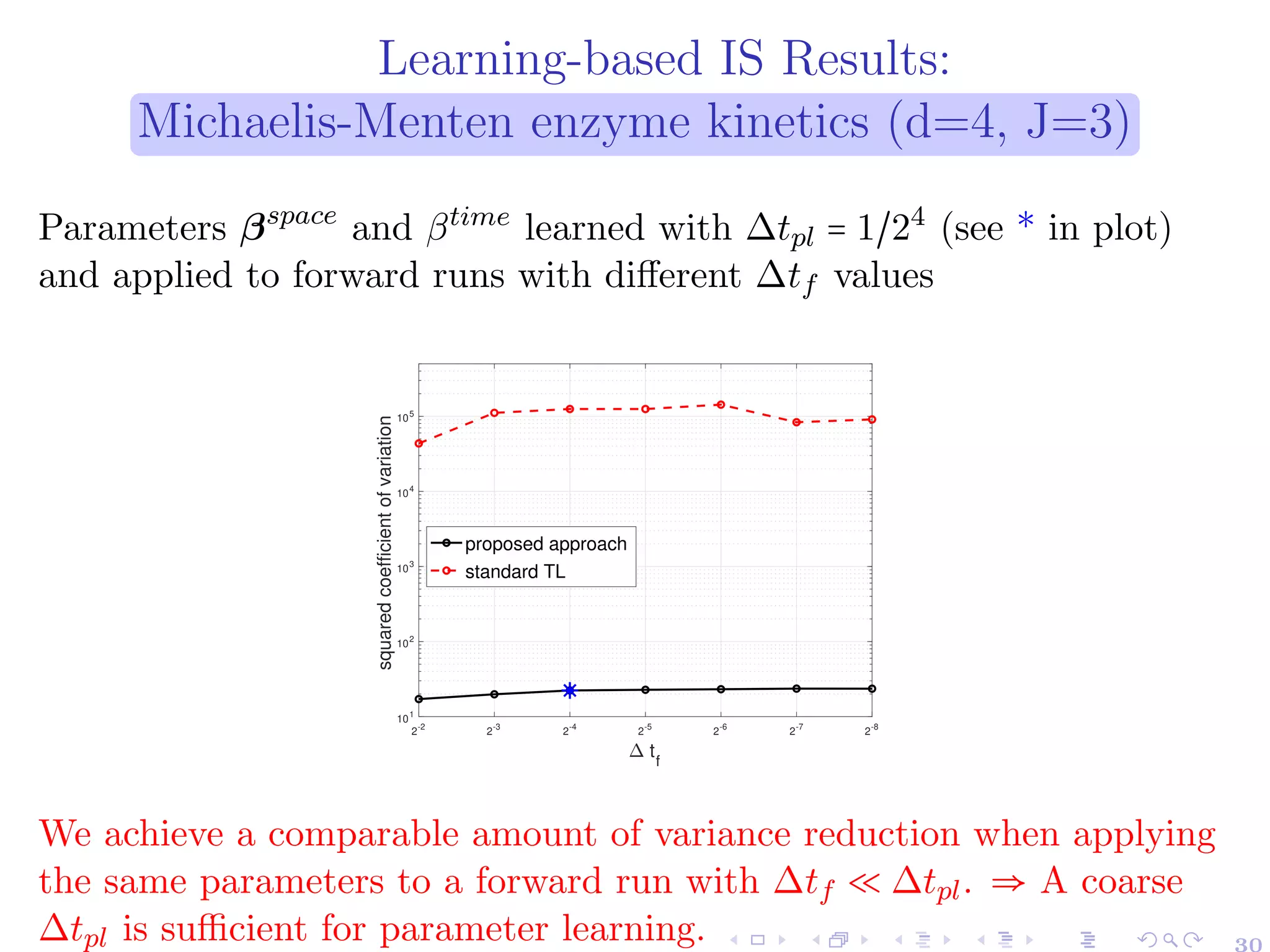
17](https://image.slidesharecdn.com/kausttalkshort-230531154446-ae89ff73/75/KAUST_talk_short-pdf-21-2048.jpg)
![Learning-Based Approach: Steps
2 Use stochastic optimization (e.g. ADAM (Kingma et al. 2014))
to learn the parameters β = (βspace
,βtime
) ∈ Rd+1
which minimize
the second moment under IS:
inf
β∈Rd+1
E[g2
(X
∆t,β
N )
N−1
∏
k=0
L2
k (P̄ k,δ̂
∆t
(k,X
∆t,β
k ;β))]
´¹¹¹¹¹¹¹¹¹¹¹¹¹¹¹¹¹¹¹¹¹¹¹¹¹¹¹¹¹¹¹¹¹¹¹¹¹¹¹¹¹¹¹¹¹¹¹¹¹¹¹¹¹¹¹¹¹¹¹¹¹¹¹¹¹¹¹¹¹¹¹¹¹¹¹¹¹¹¹¹¹¹¹¹¹¹¹¹¹¹¹¹¹¹¹¹¹¹¹¹¹¹¹¹¹¹¹¹¹¹¹¹¹¹¹¹¹¹¹¹¹¹¹¹¹¹¹¹¹¹¹¹¹¹¹¹¹¹¹¹¹¹¹¹¹¹¹¹¹¹¹¹¹¹¹¹¹¹¹¹¹¹¸¹¹¹¹¹¹¹¹¹¹¹¹¹¹¹¹¹¹¹¹¹¹¹¹¹¹¹¹¹¹¹¹¹¹¹¹¹¹¹¹¹¹¹¹¹¹¹¹¹¹¹¹¹¹¹¹¹¹¹¹¹¹¹¹¹¹¹¹¹¹¹¹¹¹¹¹¹¹¹¹¹¹¹¹¹¹¹¹¹¹¹¹¹¹¹¹¹¹¹¹¹¹¹¹¹¹¹¹¹¹¹¹¹¹¹¹¹¹¹¹¹¹¹¹¹¹¹¹¹¹¹¹¹¹¹¹¹¹¹¹¹¹¹¹¹¹¹¹¹¹¹¹¹¹¹¹¹¹¹¹¹¹
=∶C0,X (δ̂
∆t
0 ,...,δ̂
∆t
N−1;β)
,
▸ (δ̂
∆t
(n,x;β))
j
= δ̂∆t
j (n,x;β) =
aj (x)
√
û∆t(
(n+1)∆t
T ,max(0,x+νj );β)
√
û∆t(
(n+1)∆t
T ,x;β)
▸ {X
∆t,β
n }n=1,...,N is an IS path generated with {δ̂
∆t
(n,x;β)}n=1,...,N
(+) We derive explicit pathwise derivatives, which are unbiased,
resulting in only the MC error for evaluating the expectation (i.e.,
without additional finite difference error).
18](https://image.slidesharecdn.com/kausttalkshort-230531154446-ae89ff73/75/KAUST_talk_short-pdf-22-2048.jpg)

![Learning-Based Approach: Steps
3 In the forward step, estimate E[g(X(T))] using the MC estimator
based on the proposed IS change of measure over M paths
µIS
M,∆t =
1
M
M
∑
i=1
Lβ∗
i ⋅ g(X
∆t,β∗
[i],N ),
where X
∆t,β∗
[i],N is the i-th IS sample path and Lβ∗
i is the
corresponding likelihood factor, both simulated with the IS
parameters obtained via the stochastic optimization step
δ̂j(n,x;β∗
) =
aj(x)
√
û((n+1)∆t
T
,max(0,x + νj);β∗
)
√
û((n+1)∆t
T
,x;β∗
)
, 0 ≤ n ≤ N − 1, x ∈ Nd
,
,1 ≤ j ≤ J
20](https://image.slidesharecdn.com/kausttalkshort-230531154446-ae89ff73/75/KAUST_talk_short-pdf-24-2048.jpg)
![HJB equations for IS Parameters
of the full-dimensional SRNs
Corollary (Ben Hammouda et al. 2023a)
For x ∈ Nd
, an approximate continuous-time value function ũ(t,x) fulfills the
Hamilton-Jacobi-Bellman (HJB) equations for t ∈ [0,T]
ũ(T,x) = g2
(x)
−
dũ
dt
(t,x) = inf
δ(t,x)∈Ax
⎛
⎝
−2
J
∑
j=1
aj(x) +
J
∑
j=1
δj(t,x)
⎞
⎠
ũ(t,x) +
J
∑
j=1
aj(x)2
δj(t,x)
ũ(t,max(0,x + νj)),
where δj(t,x) ∶= (δ(t,x))j.
For If ũ(t,x) > 0 for all x ∈ Nd
and t ∈ [0,T] :
▸ δ̃j(t,x) = aj(x)
√
ũ(t,max(0,x+νj ))
ũ(t,x)
▸ dũ
dt
(t,x) = −2∑
J
j=1 aj(x)(
√
ũ(t,x)ũ(t,max(0,x + νj)) − ũ(t,x))
For rare event probabilities, we approximate the observable g(x) = 1xi>γ
by a sigmoid: g̃(x) = 1
1+exp(b−βxi), with appropriately chosen parameters
b ∈ R and β ∈ R.
⊖ Computational cost to solve HJB Equ. scales exponentially with dimension
d.](https://image.slidesharecdn.com/kausttalkshort-230531154446-ae89ff73/75/KAUST_talk_short-pdf-26-2048.jpg)

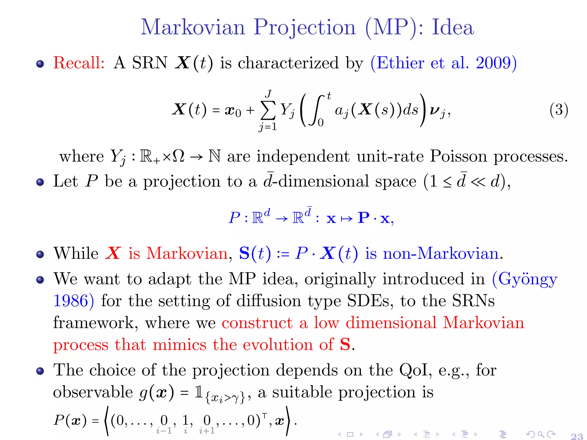
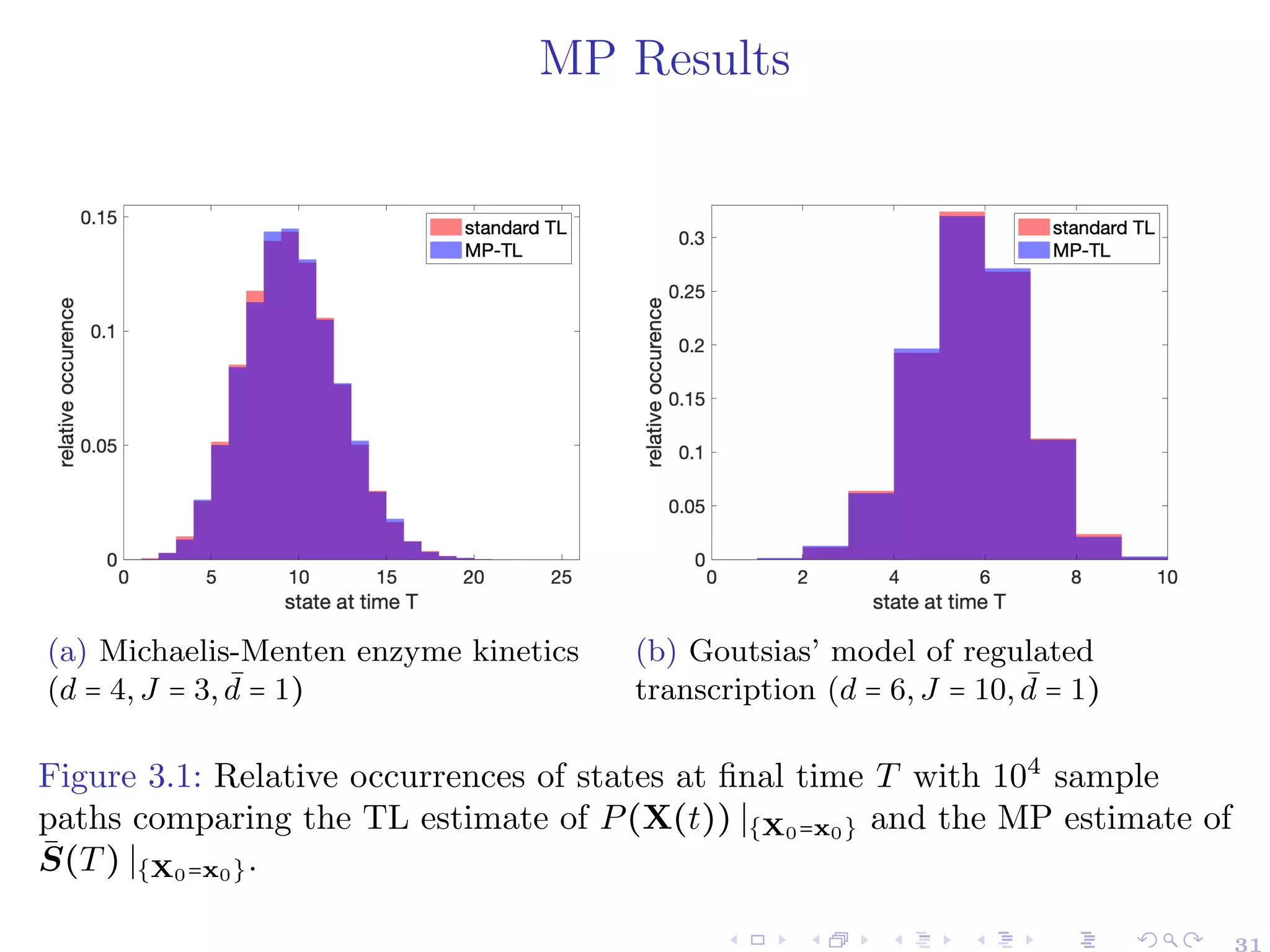
![Markovian Projection for SRNs
For t ∈ [0,T], let us consider the projected process as S(t) ∶= P ⋅ X(t),
where X(t) follows (3).
Theorem ((Ben Hammouda et al. 2023a))
For t ∈ [0,T], let S̄(t) be a ¯
d-dimensional stochastic process, whose
dynamics are given by
S̄(t) = P(x0) +
J
∑
j=1
Ȳj (∫
t
0
āj(τ,S̄(τ))dτ)P(νj)
´¹¹¹¹¹¹¸¹¹¹¹¹¹
=∶ν̄j
,
where Ȳj are independent unit-rate Poisson processes and āj are
characterized by
āj(t,s) ∶= E[aj(X(t))∣P (X(t)) = s,X(0) = x0], for 1 ≤ j ≤ J,s ∈ N
¯
d
.
Then, S(t) ∣{X(0)=x0} and S̄(t) ∣{X(0)=x0} have the same conditional
distribution for all t ∈ [0,T].
24](https://image.slidesharecdn.com/kausttalkshort-230531154446-ae89ff73/75/KAUST_talk_short-pdf-29-2048.jpg)
![Propensities of the Projected Process
Under MP, the propensity becomes time-dependent
āj(t,s) ∶= E[aj(X(t)) ∣ P (X(t)) = s;X(0) = x0], for 1 ≤ j ≤ J,s ∈ N
¯
d
The index set of the projected propensities is (#JMP ≤ J)
JMP ∶= {1 ≤ j ≤ J ∶ P(νj) ≠ 0 and aj(x) ≠ f(P(x)) ∀f ∶ R
¯
d
→ R}.
To approximate āj for j ∈ JMP , we use discrete L2
regression:
āj(⋅,⋅) = argminh∈V ∫
T
0
E[(aj(X(t)) − h(t,P(X(t))))
2
]dt
≈ argminh∈V
1
M
M
∑
m=1
1
N
N−1
∑
n=0
(aj(X̂∆t
[m],n) − h(tn,P(X̂∆t
[m],n)))
2
▸ V ∶= {f ∶ [0,T] × R
¯
d
→ R ∶ ∫
T
0 E[f(t,P(X(t))2
)]dt < ∞}
▸ {X̂∆t
[m]}
M
m=1
are M independent TL paths on a uniform time grid
0 = t0 < t1 < ⋅⋅⋅ < tN = T with step size ∆t.
25](https://image.slidesharecdn.com/kausttalkshort-230531154446-ae89ff73/75/KAUST_talk_short-pdf-30-2048.jpg)
![IS for SRNs via MP: Steps
1 Perform the MP as described in the previous slides
2 For t ∈ [0,T], solve the reduced-dimensional HJB equations
(system of ODEs) corresponding to the MP process
ũ¯
d(T,s) = g̃2
(s), s ∈ N
¯
d
dũ¯
d
dt
(t,s) = −2
J
∑
j=1
āj(t,s)(
√
ũ¯
d(t,s)ũ¯
d(t,max(0,s + ν̄j)) − ũ¯
d(t,s)), s ∈ N
¯
d
.
3 Obtain the continuous-time IS controls for the d-dimensional SRN
δ̄j(t,x) = aj(x)
¿
Á
Á
Àũ¯
d (t,max(0,P(x + νj)))
ũ¯
d (t,P(x))
, for x ∈ Nd
,t ∈ [0,T].
4 Construct the MP-IS-MC estimator for a given uniform time grid
0 = t0 ≤ t1 ≤ ⋅⋅⋅ ≤ tN = T with stepsize ∆t, with TL paths using the
IS control parameters δ̄j(tn,x), j = 1,...,J,x ∈ Nd
,n = 0,...,N − 1.
26](https://image.slidesharecdn.com/kausttalkshort-230531154446-ae89ff73/75/KAUST_talk_short-pdf-31-2048.jpg)


![Related References
Thank you for your attention!
[1] C. Ben Hammouda, N. Ben Rached, R. Tempone, S. Wiechert. Automated
Importance Sampling via Optimal Control for Stochastic Reaction
Networks: A Markovian Projection-based Approach. To appear soon (2023).
[2] C. Ben Hammouda, N. Ben Rached, R. Tempone, S. Wiechert.
Learning-based importance sampling via stochastic optimal control for
stochastic reaction networks. Statistics and Computing, 33, no. 3 (2023).
[3] C. Ben Hammouda, N. Ben Rached, R. Tempone. Importance sampling for
a robust and efficient multilevel Monte Carlo estimator for stochastic
reaction networks. Statistics and Computing, 30, no. 6 (2020).
[4] C. Ben Hammouda, A. Moraes, R. Tempone. Multilevel hybrid split-step
implicit tau-leap. Numerical Algorithms, 74, no. 2 (2017).
36](https://image.slidesharecdn.com/kausttalkshort-230531154446-ae89ff73/75/KAUST_talk_short-pdf-45-2048.jpg)
![References I
[1] David F Anderson. “A modified next reaction method for simulating chemical
systems with time dependent propensities and delays”. In: The Journal of chemical
physics 127.21 (2007), p. 214107.
[2] David F Anderson and Thomas G Kurtz. Stochastic analysis of biochemical systems.
Springer, 2015.
[3] C. Ben Hammouda et al. “Automated Importance Sampling via Optimal Control for
Stochastic Reaction Networks: A Markovian Projection-based Approach”. In: To
appear soon (2023).
[4] C. Ben Hammouda et al. “Learning-based importance sampling via stochastic
optimal control for stochastic reaction networks”. In: Statistics and Computing 33.3
(2023), p. 58.
[5] Chiheb Ben Hammouda, Alvaro Moraes, and Raúl Tempone. “Multilevel hybrid
split-step implicit tau-leap”. In: Numerical Algorithms 74.2 (2017), pp. 527–560.
[6] Chiheb Ben Hammouda, Nadhir Ben Rached, and Raúl Tempone. “Importance
sampling for a robust and efficient multilevel Monte Carlo estimator for stochastic
reaction networks”. In: Statistics and Computing 30.6 (2020), pp. 1665–1689.
[7] Corentin Briat, Ankit Gupta, and Mustafa Khammash. “A Control Theory for
Stochastic Biomolecular Regulation”. In: SIAM Conference on Control Theory and
its Applications. SIAM. 2015.
37](https://image.slidesharecdn.com/kausttalkshort-230531154446-ae89ff73/75/KAUST_talk_short-pdf-46-2048.jpg)
![References II
[8] Nai-Yuan Chiang, Yiqing Lin, and Quan Long. “Efficient propagation of
uncertainties in manufacturing supply chains: Time buckets, L-leap, and multilevel
Monte Carlo methods”. In: Operations Research Perspectives 7 (2020), p. 100144.
[9] Stewart N Ethier and Thomas G Kurtz. Markov processes: characterization and
convergence. Vol. 282. John Wiley & Sons, 2009.
[10] D. T. Gillespie. “Approximate accelerated stochastic simulation of chemically
reacting systems”. In: Journal of Chemical Physics 115 (July 2001), pp. 1716–1733.
doi: 10.1063/1.1378322.
[11] Daniel Gillespie. “Approximate accelerated stochastic simulation of chemically
reacting systems”. In: The Journal of chemical physics 115.4 (2001), pp. 1716–1733.
[12] Daniel T Gillespie. “A general method for numerically simulating the stochastic time
evolution of coupled chemical reactions”. In: Journal of computational physics 22.4
(1976), pp. 403–434.
[13] John Goutsias. “Quasiequilibrium approximation of fast reaction kinetics in
stochastic biochemical systems”. In: The Journal of chemical physics 122.18 (2005),
p. 184102.
[14] John Goutsias and Garrett Jenkinson. “Markovian dynamics on complex reaction
networks”. In: Physics reports 529.2 (2013), pp. 199–264.
38](https://image.slidesharecdn.com/kausttalkshort-230531154446-ae89ff73/75/KAUST_talk_short-pdf-47-2048.jpg)
![References III
[15] István Gyöngy. “Mimicking the one-dimensional marginal distributions of processes
having an Itô differential”. In: Probability theory and related fields 71.4 (1986),
pp. 501–516.
[16] SebastianC. Hensel, JamesB. Rawlings, and John Yin. “Stochastic Kinetic Modeling
of Vesicular Stomatitis Virus Intracellular Growth”. English. In: Bulletin of
Mathematical Biology 71.7 (2009), pp. 1671–1692. issn: 0092-8240.
[17] H. Solari J. Aparicio. “Population dynamics: Poisson approximation and its relation
to the langevin process”. In: Physical Review Letters (2001), p. 4183.
[18] Hye-Won Kang and Thomas G Kurtz. “Separation of time-scales and model
reduction for stochastic reaction networks”. In: (2013).
[19] Diederik P Kingma and Jimmy Ba. “Adam: A method for stochastic optimization”.
In: arXiv preprint arXiv:1412.6980 (2014).
[20] Hiroyuki Kuwahara and Ivan Mura. “An efficient and exact stochastic simulation
method to analyze rare events in biochemical systems”. In: The Journal of chemical
physics 129.16 (2008), 10B619.
[21] Christopher V Rao and Adam P Arkin. “Stochastic chemical kinetics and the
quasi-steady-state assumption: Application to the Gillespie algorithm”. In: The
Journal of chemical physics 118.11 (2003), pp. 4999–5010.
39](https://image.slidesharecdn.com/kausttalkshort-230531154446-ae89ff73/75/KAUST_talk_short-pdf-48-2048.jpg)
![References IV
[22] Elijah Roberts et al. “Noise Contributions in an Inducible Genetic Switch: A
Whole-Cell Simulation Study”. In: PLoS computational biology 7 (Mar. 2011),
e1002010. doi: 10.1371/journal.pcbi.1002010.
[23] Sophia Wiechert. “Optimal Control of Importance Sampling Parameters in Monte
Carlo Estimators for Stochastic Reaction Networks”. MA thesis. 2021.
40](https://image.slidesharecdn.com/kausttalkshort-230531154446-ae89ff73/75/KAUST_talk_short-pdf-49-2048.jpg)

The document discusses the design of efficient Monte Carlo estimators for rare event probabilities in stochastic reaction networks using optimal importance sampling via stochastic optimal control. Two approaches are explored: a learning-based method for the value function and controls through stochastic optimization, and a Markovian projection-based method for solving reduced-dimensional Hamilton-Jacobi-Bellman equations. The goal is to address challenges like the curse of dimensionality while providing numerical experiments and results to support these methodologies.