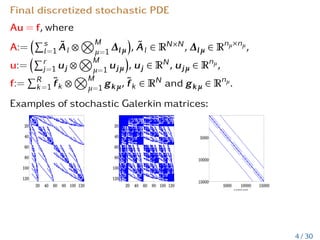
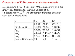
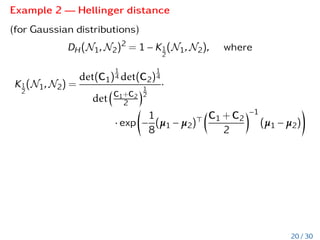
This document discusses the computation of f-divergences and distances for high-dimensional probability density functions (PDFs) using techniques from stochastic analysis, such as Karhunen-Loève and polynomial chaos expansions. It highlights methods for calculating Kullback-Leibler divergence and other entropy measures when PDFs are either unknown or do not exist. Additionally, it presents various algorithms, tensor representations, and numerical examples to demonstrate the computational efficiency and effectiveness of the approaches presented.

1. Computing f-Divergences and Distances of
High-Dimensional Probability Density Functions
Alexander Litvinenko (RWTH Aachen, Germany),
joint work with
Youssef Marzouk, Hermann G. Matthies, Marco Scavino, Alessio Spantini
SIAM IS 2022

2. Plan
1. Motivating examples, working diagram
2. Basics: pdf, cdf, FFT
3. Theoretical background
4. Computation of moments and divergences
5. Tensor formats
6. Algorithms
7. Numerics
1 / 30

3. Motivation and settings:
Assume we use Karhunen-Loeve and (or) Polynomial Chaos
Expansion methods to solve
1. a PDE with uncertain coefficients,
2. a parameter inference problem,
3. a data assimilation task,
4. an optimal design of experiment task.
As a result, we obtain a functional representation (KLE, PCE) of
our uncertain QoI.
How to compute KLD and other divergences? (Classical result
is given only for pdfs, which are not known).
How to compute entropy, KLD and other divergences if pdfs are
not available or not exist?
2 / 30

4. Motivation: stochastic PDEs
−∇ · (κ(x,ω)∇u(x,ω)) = f(x,ω), x ∈ G ⊂ Rd
, ω ∈ Ω
Write first Karhunen-Loeve Expansion and then for
uncorrelated random variables the Polynomial Chaos
Expansion
u(x,ω) =
K
X
i=1
p
λiφi(x)ξi(ω) =
K
X
i=1
p
λiφi(x)
X
α∈J
ξ
(α)
i Hα(θ(ω))
(1)
where ξ
(α)
i is a tensor. Note that α = (α1,α2,...,αM,...) is a
multi-index.
X
α∈J
ξ
(α)
i Hα(θ(ω)) :=
p1
X
α1=1
...
pM
X
αM=1
ξ
(α1,...,αM)
i
M
Y
j=1
hαj
(θj) (2)
The same decomposition for κ(x,ω).
3 / 30

5. Final discretized stochastic PDE
Au = f, where
A:=
Ps
l=1 Ãl ⊗
NM
µ=1 ∆lµ
, Ãl ∈ RN×N, ∆lµ ∈ Rnµ×nµ,
u:=
Pr
j=1 uj ⊗
NM
µ=1 ujµ
, uj ∈ RN, ujµ ∈ Rnµ,
f:=
PR
k=1 f̃k ⊗
NM
µ=1 gkµ, f̃k ∈ RN and gkµ ∈ Rnµ.
Examples of stochastic Galerkin matrices:
4 / 30

6. How to compute KLE, divergences if pdf is not available?
Two ways to compute f-divergence, KLD, entropy.
5 / 30

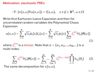
7. Connection of pcf and pdf
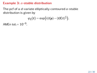
The probability characteristic function (pcf ) ϕξ could be
defined:
ϕξ(t) := E(exp(ihξ|ti)) :=
Z
Rd
pξ(y)exp(ihy|ti) dy =: F [d]
(pξ)(t),
where t = (t1,t2,...,td) ∈ Rd is the dual variable to y ∈ Rd,
hy|ti =
Pd
j=1 yjtj is the canonical inner product on Rd, and F [d]
is the probabilist’s d-dimensional Fourier transform.
pξ(y) =
1
(2π)d
Z
Rd
exp(−iht|yi)ϕξ(t)dt = F [−d]
(ϕξ)(y). (3)
6 / 30

8. Discrete low-rank representation of pcf
We try to find an approximation
ϕξ(t) ≈ e
ϕξ(t) =
R
X
`=1
d
O
ν=1
ϕ`,ν(tν), (4)
where the ϕ`,ν(tν) are one-dimensional functions.
Then we can get
pξ(y) ≈ e
pξ(y) = F [−d]
(ϕξ)y =
R
X
`=1
d
O
ν=1
F −1
1 (ϕ`,ν)(yν),
where F −1
1 is the one-dimensional inverse Fourier transform.
7 / 30

9. Representation of a 3D tensor in the CP tensor format
A full tensor w ∈ Rn1×n2×n3 (on the left) is represented as a sum
of tensor products. The lines on the right denote vectors
wi,k ∈ Rnk , i = 1,...,r, k = 1,2,3.
8 / 30

10. CP tensor format linear algebra
α · w =
r
X
j=1
α
d
O
ν=1
wj,ν =
r
X
j=1
d
O
ν=1
ανwj,ν
where αν := d
√
|α| for all ν 1. and α1 := sign(α) d
√
|α|.
The sum of two tensors costs only O(1):
w = u + v =








ru
X
j=1
d
O
ν=1
uj,ν








+









rv
X
k=1
d
O
µ=1
vk,µ









=
ru+rv
X
j=1
d
O
ν=1
wj,ν
where wj,ν := uj,ν for j ≤ ru and wj,ν := vj,ν for ru j ≤ ru + rv.
The sum w generally has rank ru + rv.
9 / 30

11. CP properties: Hadamard product
u

12. v =








ru
X
j=1
d
O
ν=1
uj,ν









13. 






rv
X
k=1
d
O
ν=1
vk,ν






 =
ru
X
j=1
rv
X
k=1
d
O
ν=1
(uj,ν

14. vk,ν)
The new rank can increase till rurv, and the computational cost
is O(ru rvn d).
The scalar product can be computed as follows:
hu|viT = h
ru
X
j=1
d
O
ν=1
uj,ν|
rv
X
k=1
d
O
ν=1
vk,νiT =
ru
X
j=1
rv
X
k=1
d
Y
ν=1
huj,ν|vk,νi
Cost is O(ru rv n d).
Rank truncation via the ALS-method or Gauss-Newton-method.
The scalar product above helps to compute the Frobenius norm
kuk2 :=
p
hu|viT .
10 / 30

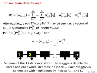
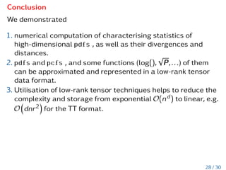
15. Tensor Train data format
w := (wi1...id
) =
r0
X
j0=1
...
rd
X
jd=1
w
(1)
j0j1
[i1]···w
(ν)
jν−1jν
[iν]···w
(d)
jd−1jd
[id]
Alternatively, each TT-core W(ν)
may be seen as a vector of
rν−1 × rν matrices W
(ν)
iν
of length Mν, i.e.
W(ν)
= (W
(ν)
iν
) : 1 ≤ iν ≤ Mν. Then
w := (wi1...id
) =
d
Y
ν=1
W
(ν)
iν
.
Schema of the TT decomposition. The waggons denote the TT
cores and each wheel denotes the index iν. Each waggon is
connected with neighbours by indices jν−1 and jν. 11 / 30

16. Computation of QoIs
Z
p(x) dx ≈ S(P) :=
V
N
hP|iT .
E(f(ξ)) =
Z
Rd
f(x)pξ(x) dx ≈ S(F

17. P) =
V
N
hF|PiT
Differential entropy, requiring the point-wise logarithm of P:
h(p) := E(−log(p))p ≈ E(−log(P))P = −
V
N
hlog(P)|Pi,
Then the f-divergence of p from q and its discrete
approximation is defined as
Df(pkq) := E f
p
q
!!
q
≈ E
f(P

18. Q

19. −1
)
Q
=
V
N
hf(P

20. Q

21. −1
)|Qi.
12 / 30

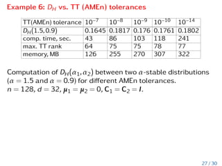
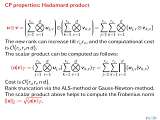
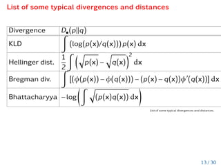
22. List of some typical divergences and distances
Divergence D•(pkq)
KLD
Z
(log(p(x)/q(x)))p(x) dx
Hellinger dist.
1
2
Z q
p(x) −
q
q(x)
2
dx
Bregman div.
Z
[(φ(p(x)) − φ(q(x))) − (p(x) − q(x))φ0
(q(x))] dx
Bhattacharyya −log
Z q
(p(x)q(x)) dx
!
List of some typical divergences and distances.
13 / 30

23. Discrete approximations for divergences
Divergence Approx. D•(pkq)
KLD
V
N
(hlog(P)|Pi − hlog(Q)|Pi)
(DH)2:
V
2N
hP

24. 1/2
− Q

25. 1/2
|P

26. 1/2
− Q

27. 1/2
i
Dφ: S ((φ(P) − φ(Q)) − (P − Q)

28. φ0
(Q))
DBh: −log
V
N
hP

29. 1/2
|Q

30. 1/2
i
14 / 30

31. Computing pointwise inverse w