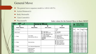
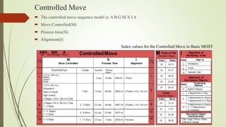
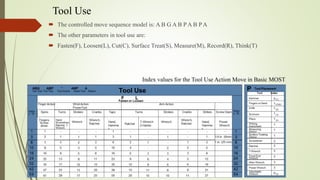
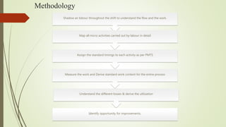
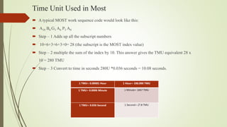
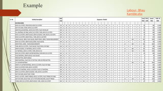
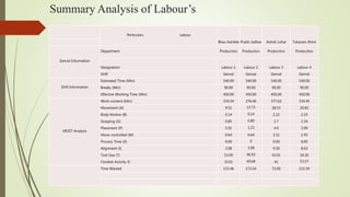
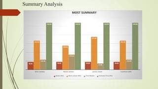
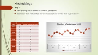
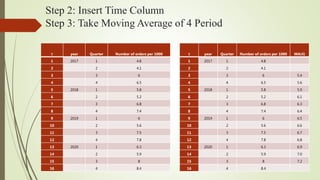
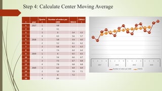
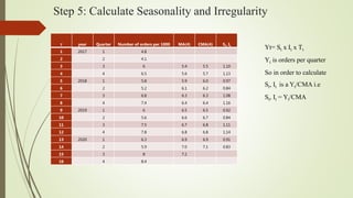
The document discusses productivity improvement through Maynard's Operation Sequence Technique (MOST) and time series forecasting, detailing the methodology for time studies, standard work content measurement, and workload analysis for labor across various tasks. It includes a summary of individual laborers' work effectiveness, their time wastage, suggestions for improvement, and a time series analysis of quarterly order data with trends and seasonality. The findings emphasize the importance of efficient workflow, minimizing waste, and forecasting to enhance productivity in a production setting.

1. Productivity Improvement by Maynards Operation Sequence
Technique & Time Series Forecasting
By
Mr. Gajanan Pathak
M. Tech II Year
119M0078
Prof. Prakash Vaidya
Prof. Suvarna Mane
Guides
Dr. G. N. Kotwal
H.O.D

2. What is time Study?

3. Maynard Operation Sequence Technique (MOST®)
 Considered a revolutionary Predetermined Motion Time System(PMTS)
 Developed by Kjell Zandin and H. B. Maynard and Company, Inc. in 1974
 MOST® times represent ranges of motions.
 Very accurate results are produced because ranges are statistically derived.
 Based on Methods Time Measurement(MTM).

4. Sequence Model and Terminology
Activity Sequence Model Parameter
General Move A B G A B PA A= Action Distance
B= Body Motion
G= Gain control
P= Placement
Controlled Move A B G M X I A M= Move Controlled
X= Process Time
I= Alignment
Tool Use A B G A B P A B P A F= Fasten
L= Loosen
C= Cut
S= Surface Treat
M= Measure
R= Record
T= Think

5. General Move
 The general move sequence model is: A B G A B P A
 Action Distance(A)
 Body Motion(B)
 Gain Control(G)
 Placement(P) Index values for the General Move in Basic MOST

6. Controlled Move
 The controlled move sequence model is: A B G M X I A
 Move Controlled(M)
 Process time(X)
 Alignment(I)
Index values for the Controlled Move in Basic MOST

7. Tool Use
 The controlled move sequence model is: A B G A B P A B P A
 The other parameters in tool use are:
 Fasten(F), Loosen(L), Cut(C), Surface Treat(S), Measure(M), Record(R), Think(T)
Index values for the Tool Use Action Move in Basic MOST

8. Methodology
Shadow an lobour throughout the shift to understand the flow and the work.
Map all micro activities carried out by labour in detail
Assign the standard timings to each activity as per PMTS
Measure the work and Derive standard work content for the entire process
Understand the different losses & derive the utilization
Identify opportunity for improvements.

9. Time Unit Used in Most
 A typical MOST work sequence code would look like this:
 A10 B6 G3 A6 P3 A0
 Step – 1 Adds up all the subscript numbers
 10+6+3+6+3+0= 28 (the subscript is the MOST index value)
 Step – 2 multiple the sum of the index by 10. This answer gives the TMU equivalent 28 x
10 = 280 TMU
 Step – 3 Convert to time in seconds 280U *0.036 seconds = 10.08 seconds.
1 TMU= 0.00001 Hour 1 Hour= 100,000 TMU
1 TMU= 0.0006 Minute 1 Minute= 1667 TMU
1 TMU= 0.036 Second 1 Second= 27.8 TMU

10. Example
Labour- Bhau
Kamble.xlsx

11. Summary Analysis of Labour’s
Perticulars Labour
Bhau Kamble Pratik Jadhav Ashok Lohar Tukaram Ahire
Genral Information
Department Production Production Production Production
Designation Labour 1 Labour 2 Labour 3 Labour 4
Shift Genral Genral Genral Genral
Shift Information
Estimated Time (Min) 540.00 540.00 540.00 540.00
Breaks (Min) 90.00 90.00 90.00 90.00
Effective Working Time (Min) 450.00 450.00 450.00 450.00
MOST Analysis
Work content (Min) 334.54 276.46 377.62 334.45
Movement (A) 9.51 13.73 28.53 20.82
Body Motion (B) 0.14 0.14 2.22 2.10
Grasping (G) 0.85 0.89 2.7 2.34
Placement (P) 5.91 1.23 4.4 3.99
Move controlled (M) 0.64 0.64 2.11 1.93
Process Time (X) 0.00 0 0.00 0.00
Alignment (I) 3.08 3.08 9.30 8.63
Tool Use (T) 53.09 46.93 43.01 34.26
Clocked Activity © 33.01 49.68 41 53.57
Time Wasted 115.46 173.54 72.00 115.59

12. Summary Analysis
90.00 90.00 90.00 90.00
334.54
276.46
377.62
334.45
115.46
173.54
72.00
115.59
540.00 540.00 540.00 540.00
BHAU KAMBLE PRATIK JADHAV ASHOK LOHAR TUKARAM AHIRE
MOST SUMMARY
Breaks (Min) Work content (Min) Time Wasted Estimated Time (Min)

13. Average of MOST Summary
Bhau
Kamble
Pratik
Jadhav
Ashok
Lohar
Tukaram
Ahire
Breaks (Min) 90.00 90.00 90.00 90.00
Work content (Min) 334.54 276.46 377.62 334.45
Time Wasted 115.46 173.54 72.00 115.59
Estimated Time (Min) 540.00 540.00 540.00 540.00
Breaks (Min) 90.00
Work content (Min) 330.77
Time Wasted 119.15
Estimated Time (Min) 540.00
Average of MOST Summary
MOST Summary
90.00
330.77
119.15
540.00
BREAKS (MIN) WORK CONTENT
(MIN)
TIME WASTED ESTIMATED TIME
(MIN)
Average of MOST Summary
Breaks (Min)
Work content (Min)
Time Wasted
Estimated Time (Min)

14. Summary of All Micro Activities of Each Labour’s
Movement (A), 9.51, 9%
Body Motion (B), 0.14, 0%
Grasping (G), 0.85, 1%
Placement (P), 5.91, 5%
Move controlled (M), 0.64, 1%
Process Time (X), 0.00, 0%
Alignment (I), 3.08, 3%
Tool Use (T), 53.09, 50%
Clocked Activity ©, 33.01, 31%
Labour 1- Bhau Kamble
Movement (A)
Body Motion (B)
Grasping (G)
Placement (P)
Move controlled (M)
Process Time (X)
Alignment (I)
Tool Use (T)
Clocked Activity ©

15. Movement (A), 13.73, 12%
Body Motion (B), 0.14, 0%
Grasping (G), 0.89, 1%
Placement (P), 1.23, 1%
Move controlled (M), 0.64, 0%
Process Time (X), 0, 0%
Alignment (I), 3.08, 3%
Tool Use (T), 46.93, 40%
Clocked Activity ©, 49.68, 43%
Labour 2- Pratik jadhav
Movement (A)
Body Motion (B)
Grasping (G)
Placement (P)
Move controlled (M)
Process Time (X)
Alignment (I)
Tool Use (T)
Clocked Activity ©

16. Movement (A), 28.53, 21%
Body Motion (B), 2.22, 2%
Grasping (G), 2.7, 2%
Placement (P), 4.4, 3%
Move controlled (M), 2.11, 2%
Process Time (X), 0.00, 0%
Alignment (I), 9.30, 7%
Tool Use (T), 43.01, 32%
Clocked Activity ©, 41, 31%
Labour 3- Ashok Lohar
Movement (A)
Body Motion (B)
Grasping (G)
Placement (P)
Move controlled (M)
Process Time (X)
Alignment (I)
Tool Use (T)
Clocked Activity ©

17. Movement (A), 20.82, 16%
Body Motion (B), 2.10, 2%
Grasping (G), 2.34, 2%
Placement (P), 3.99, 3%
Move controlled (M), 1.93, 1%
Process Time (X), 0.00, 0%
Alignment (I), 8.63, 7%
Tool Use (T), 34.26, 27%
Clocked Activity ©, 53.57, 42%
Labour 4- Tukaram Ahire
Movement (A)
Body Motion (B)
Grasping (G)
Placement (P)
Move controlled (M)
Process Time (X)
Alignment (I)
Tool Use (T)
Clocked Activity ©

18. Observation’s
 Time is wasted for collected material for stitching belt
 Time is wasted due to long distance between machine and storage
 Time wasted for adjusting material
 More time taken for starting their work
 Time is wasted for adjusting machines
 more time taken for cutting of material
 Time is wasted due to collection of material
 more time taken for handling machines
 More Time is wasted in clocked activities

19. Result and Conclusion
Time in Min Percentage
Shift 540.00 100.00
Breaks 90.00 16.67
Effective working time 450.00 83.33
Work content by Most 377.62 69.93
Time wasted 72.38 13.40
Akash Lohar
Time in Min Percentage
Shift 540.00 100.00
Breaks 90.00 16.67
Effective working time 450.00 83.33
Work content by Most 334.54 61.95
Time wasted 115.46 21.38
Bhau Kamble
Time in Min Percentage
Shift 540.00 100.00
Breaks 90.00 16.67
Effective working time 450.00 83.33
Work content by Most 276.46 51.20
Time wasted 173.54 32.14
Pratik Jadhav
Time in Min Percentage
Shift 540.00 100.00
Breaks 90.00 16.67
Effective working time 450.00 83.33
Work content by Most 334.45 61.94
Time wasted 115.55 21.40
Tukaram Ahire

20. Improvement
 They can start their work earlier without wasting time
 They should sort their material in store room for ease of finding them
 The distance should be less between machine and storage if possible
 Less time should take for discussion and phone calls i.e. clocked activities

21. Time Series Forecasting

22. Different Time Series Component
 Trend Component
 Seasonal Component
 Residual Component

23. Methodology
 The quarterly sale of number of orders is given below:
 Create line chart with markers for visualization of data and the chart is given below:
Year Quarter Number of orders per 1000
2017 1 4.8
2 4.1
3 6
4 6.5
2018 1 5.8
2 5.2
3 6.8
4 7.4
2019 1 6
2 5.6
3 7.5
4 7.8
2020 1 6.3
2 5.9
3 8
4 8.4
Step 1:
4.8
4.1
6
6.5
5.8
5.2
6.8
7.4
6
5.6
7.5
7.8
6.3
5.9
8
8.4
1 2 3 4 1 2 3 4 1 2 3 4 1 2 3 4
2017 2018 2019 2020
Number of orders per 1000
Number of orders per 1000

24. Step 2: Insert Time Column
Step 3: Take Moving Average of 4 Period
T year Quarter Number of orders per 1000
1 2017 1 4.8
2 2 4.1
3 3 6
4 4 6.5
5 2018 1 5.8
6 2 5.2
7 3 6.8
8 4 7.4
9 2019 1 6
10 2 5.6
11 3 7.5
12 4 7.8
13 2020 1 6.3
14 2 5.9
15 3 8
16 4 8.4
T year Quarter Number of orders per 1000 MA(4)
1 2017 1 4.8
2 2 4.1
3 3 6 5.4
4 4 6.5 5.6
5 2018 1 5.8 5.9
6 2 5.2 6.1
7 3 6.8 6.3
8 4 7.4 6.4
9 2019 1 6 6.5
10 2 5.6 6.6
11 3 7.5 6.7
12 4 7.8 6.8
13 2020 1 6.3 6.9
14 2 5.9 7.0
15 3 8 7.2
16 4 8.4

25. Step 4: Calculate Center Moving Average
t year
Quarte
r
Number of orders per
1000 MA(4)
CMA(4
)
1 2017 1 4.8
2 2 4.1
3 3 6 5.4 5.5
4 4 6.5 5.6 5.7
5 2018 1 5.8 5.9 6.0
6 2 5.2 6.1 6.2
7 3 6.8 6.3 6.3
8 4 7.4 6.4 6.4
9 2019 1 6 6.5 6.5
10 2 5.6 6.6 6.7
11 3 7.5 6.7 6.8
12 4 7.8 6.8 6.8
13 2020 1 6.3 6.9 6.9
14 2 5.9 7.0 7.1
15 3 8 7.2
16 4 8.4
4.8
4.1
6
6.5
5.8
5.2
6.8
7.4
6
5.6
7.5
7.8
6.3
5.9
8
8.4
5.5
5.7
6.0
6.2 6.3 6.4 6.5 6.7 6.8 6.8 6.9 7.1
1 2 3 4 1 2 3 4 1 2 3 4 1 2 3 4
2017 2018 2019 2020
Number of orders per 1000 CMA(4)

26. Step 5: Calculate Seasonality and Irregularity
T year Quarter Number of orders per 1000 MA(4) CMA(4) St, It
1 2017 1 4.8
2 2 4.1
3 3 6 5.4 5.5 1.10
4 4 6.5 5.6 5.7 1.13
5 2018 1 5.8 5.9 6.0 0.97
6 2 5.2 6.1 6.2 0.84
7 3 6.8 6.3 6.3 1.08
8 4 7.4 6.4 6.4 1.16
9 2019 1 6 6.5 6.5 0.92
10 2 5.6 6.6 6.7 0.84
11 3 7.5 6.7 6.8 1.11
12 4 7.8 6.8 6.8 1.14
13 2020 1 6.3 6.9 6.9 0.91
14 2 5.9 7.0 7.1 0.83
15 3 8 7.2
16 4 8.4
Yt= St x It x Tt
Yt is orders per quarter
So in order to calculate
St, It is a Yt/CMA i.e
St, It = Yt/CMA

27. Step 6: Let’s Get Rid of Irregularity and
Deseasonalize the Data
T year
Quart
er
Number of orders per
1000 MA(4)
CMA(
4) St, It St
1 2017 1 4.8 0.93
2 2 4.1 0.84
3 3 6 5.4 5.5 1.10 1.09
4 4 6.5 5.6 5.7 1.13 1.14
5 2018 1 5.8 5.9 6.0 0.97 0.93
6 2 5.2 6.1 6.2 0.84 0.84
7 3 6.8 6.3 6.3 1.08 1.09
8 4 7.4 6.4 6.4 1.16 1.14
9 2019 1 6 6.5 6.5 0.92 0.93
10 2 5.6 6.6 6.7 0.84 0.84
11 3 7.5 6.7 6.8 1.11 1.09
12 4 7.8 6.8 6.8 1.14 1.14
13 2020 1 6.3 6.9 6.9 0.91 0.93
14 2 5.9 7.0 7.1 0.83 0.84
15 3 8 7.2 1.09
16 4 8.4 1.14
T year
Quar
ter
Number of
orders per 1000
MA(
4)
CMA
(4) St, It St
Deseason
alise
1 2017 1 4.8 0.93 5.1
2 2 4.1 0.84 4.9
3 3 6 5.4 5.5 1.10 1.09 5.5
4 4 6.5 5.6 5.7 1.13 1.14 5.7
5 2018 1 5.8 5.9 6.0 0.97 0.93 6.2
6 2 5.2 6.1 6.2 0.84 0.84 6.2
7 3 6.8 6.3 6.3 1.08 1.09 6.2
8 4 7.4 6.4 6.4 1.16 1.14 6.5
9 2019 1 6 6.5 6.5 0.92 0.93 6.4
10 2 5.6 6.6 6.7 0.84 0.84 6.7
11 3 7.5 6.7 6.8 1.11 1.09 6.9
12 4 7.8 6.8 6.8 1.14 1.14 6.8
13 2020 1 6.3 6.9 6.9 0.91 0.93 6.8
14 2 5.9 7.0 7.1 0.83 0.84 7.0
15 3 8 7.2 1.09 7.3
16 4 8.4 1.14 7.3

28. Step 7: Find Out Trend Component
Coefficients
Intercept 5.09961
t 0.147139
Short Summary of Simple
linear regression
T year
Quarte
r
Number of orders per
1000 MA(4)
CMA(4
) St, It St
Deseasonali
se Tt
1 2017 1 4.8 0.93 5.1 5.25
2 2 4.1 0.84 4.9 5.39
3 3 6 5.4 5.5 1.10 1.09 5.5 5.54
4 4 6.5 5.6 5.7 1.13 1.14 5.7 5.69
5 2018 1 5.8 5.9 6.0 0.97 0.93 6.2 5.84
6 2 5.2 6.1 6.2 0.84 0.84 6.2 5.98
7 3 6.8 6.3 6.3 1.08 1.09 6.2 6.13
8 4 7.4 6.4 6.4 1.16 1.14 6.5 6.28
9 2019 1 6 6.5 6.5 0.92 0.93 6.4 6.42
10 2 5.6 6.6 6.7 0.84 0.84 6.7 6.57
11 3 7.5 6.7 6.8 1.11 1.09 6.9 6.72
12 4 7.8 6.8 6.8 1.14 1.14 6.8 6.87
13 2020 1 6.3 6.9 6.9 0.91 0.93 6.8 7.01
14 2 5.9 7.0 7.1 0.83 0.84 7.0 7.16
15 3 8 7.2 1.09 7.3 7.31
16 4 8.4 1.14 7.3 7.45
Do the Simple Linear
Regression of Deseanonalize
Data for Finding the Trend
Component

29. Step 8: Forecasting the Time Series Data
T year
Quarte
r
Number of
orders per
1000
MA(4
)
CMA(4
) St, It St
Deseasonali
se Tt
Forecas
t
1 2017 1 4.8 0.93 5.1 5.25 4.89
2 2 4.1 0.84 4.9 5.39 4.52
3 3 6 5.4 5.5 1.10 1.09 5.5 5.54 6.06
4 4 6.5 5.6 5.7 1.13 1.14 5.7 5.69 6.50
5 2018 1 5.8 5.9 6.0 0.97 0.93 6.2 5.84 5.44
6 2 5.2 6.1 6.2 0.84 0.84 6.2 5.98 5.01
7 3 6.8 6.3 6.3 1.08 1.09 6.2 6.13 6.70
8 4 7.4 6.4 6.4 1.16 1.14 6.5 6.28 7.18
9 2019 1 6 6.5 6.5 0.92 0.93 6.4 6.42 5.99
10 2 5.6 6.6 6.7 0.84 0.84 6.7 6.57 5.50
11 3 7.5 6.7 6.8 1.11 1.09 6.9 6.72 7.35
12 4 7.8 6.8 6.8 1.14 1.14 6.8 6.87 7.85
13 2020 1 6.3 6.9 6.9 0.91 0.93 6.8 7.01 6.54
14 2 5.9 7.0 7.1 0.83 0.84 7.0 7.16 6.00
15 3 8 7.2 1.09 7.3 7.31 7.99
16 4 8.4 1.14 7.3 7.45 8.52
17 2021 1 0.93 7.60 7.09
18 2 0.84 7.75 6.49
19 3 1.09 7.90 8.63
20 4 1.14 8.04 9.19
4.8
4.1
6
6.5
5.8
5.2
6.8
7.4
6
5.6
7.5
7.8
6.3
5.9
8
8.4
5.5
5.7 6.0 6.2 6.3 6.4 6.5 6.7 6.8 6.8 6.9 7.1
4.89
4.52
6.06
6.50
5.44
5.01
6.70
7.18
5.99
5.50
7.35
7.85
6.54
6.00
7.99
8.52
7.09
6.49
8.63
9.19
1 2 3 4 1 2 3 4 1 2 3 4 1 2 3 4 1 2 3 4
2017 2018 2019 2020 2021
Number of orders per 1000 CMA(4) Forecast

30. Result
 So the Final Forecasted Data is given below:
Year Quarter
Forecast(Per 1000
Orders)
2021 1 7.09
2 6.49
3 8.63
4 9.19

31. Thank You