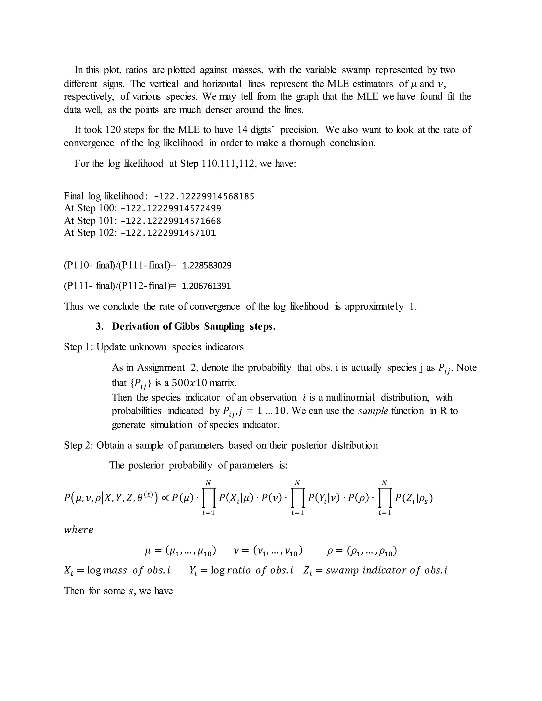
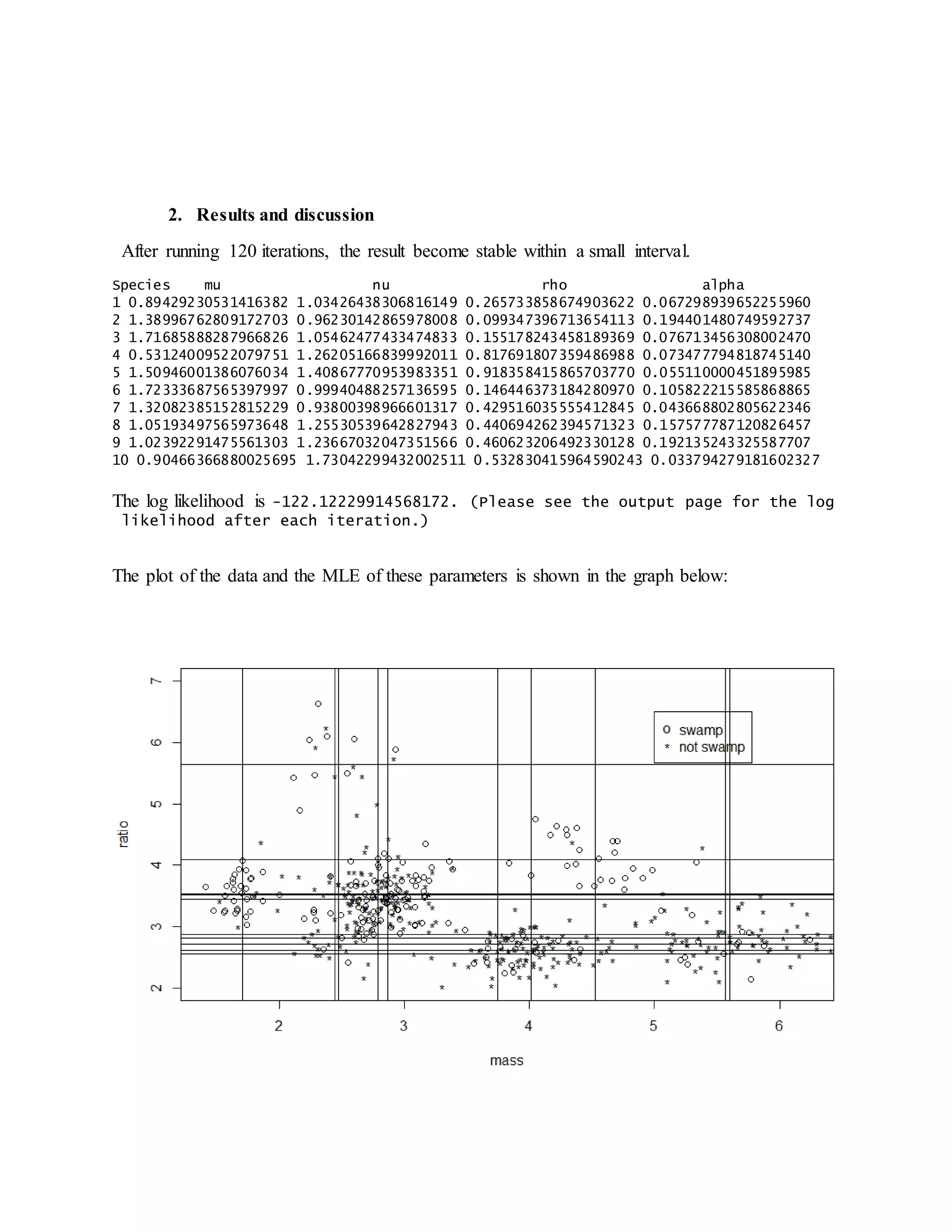
- The document describes maximum likelihood estimation (MLE) of species parameters from beetle mass, length, and other character data. - It derives EM steps to estimate species means (μ, ν), proportions (ρ), and priors (α) in the presence of missing species data. - Running the EM algorithm for 120 iterations estimates the parameters and converges the log likelihood to 14 digits of precision with a convergence rate of approximately 1. 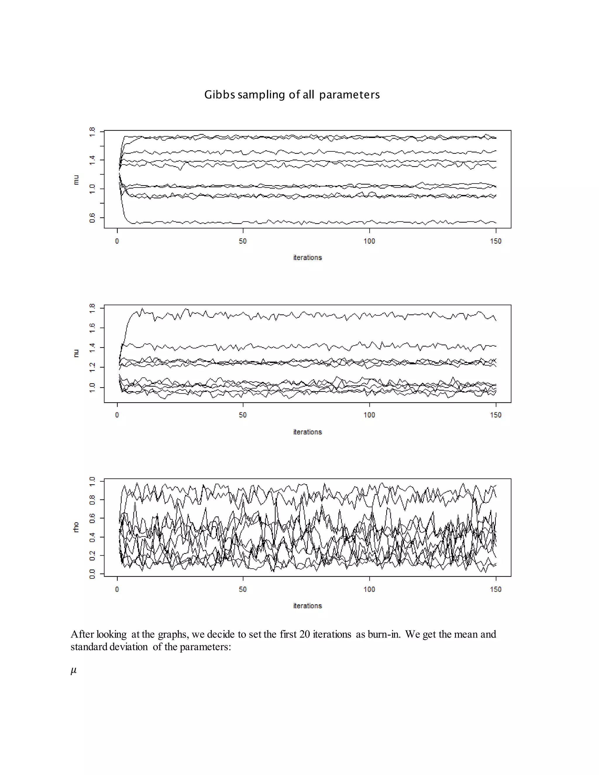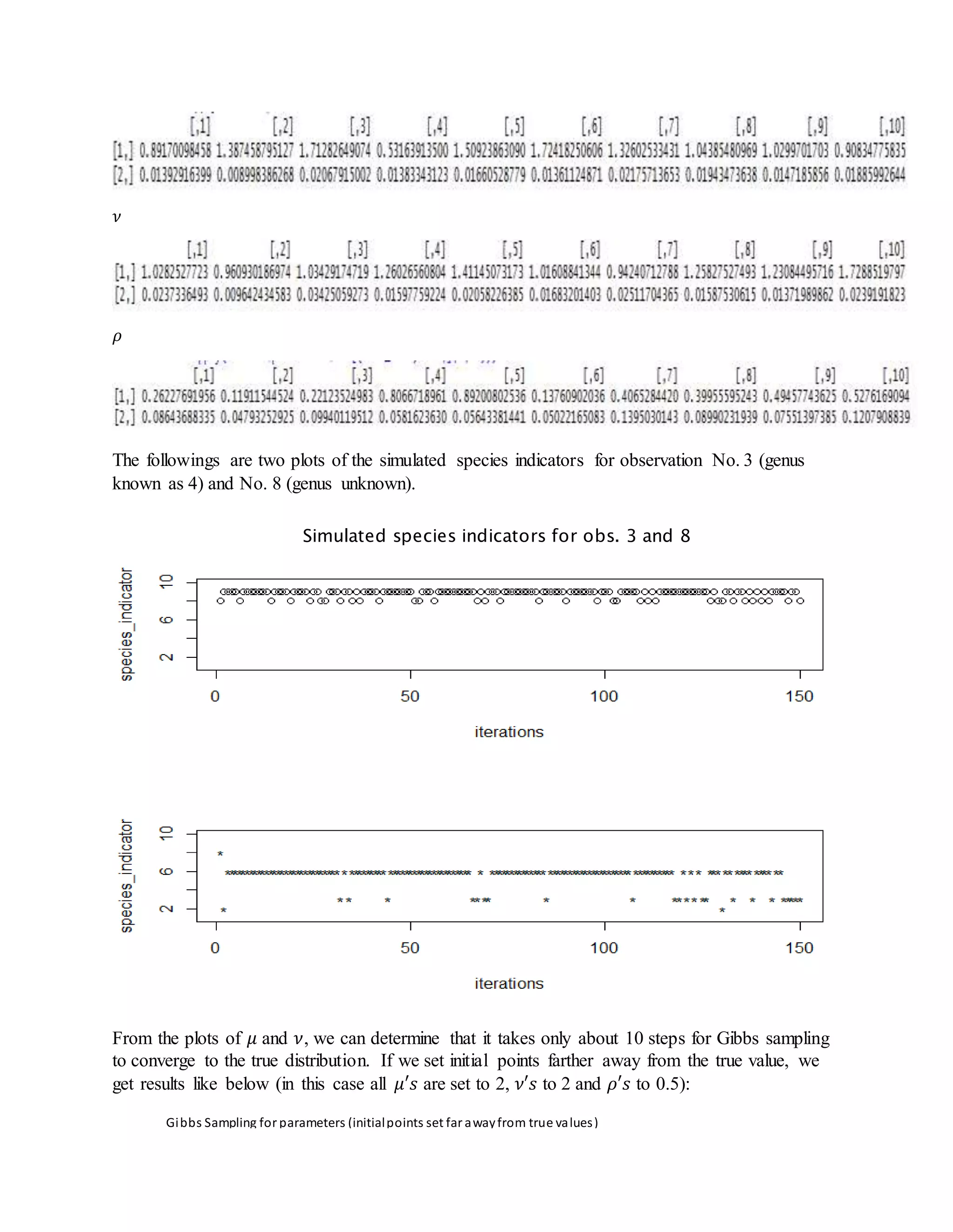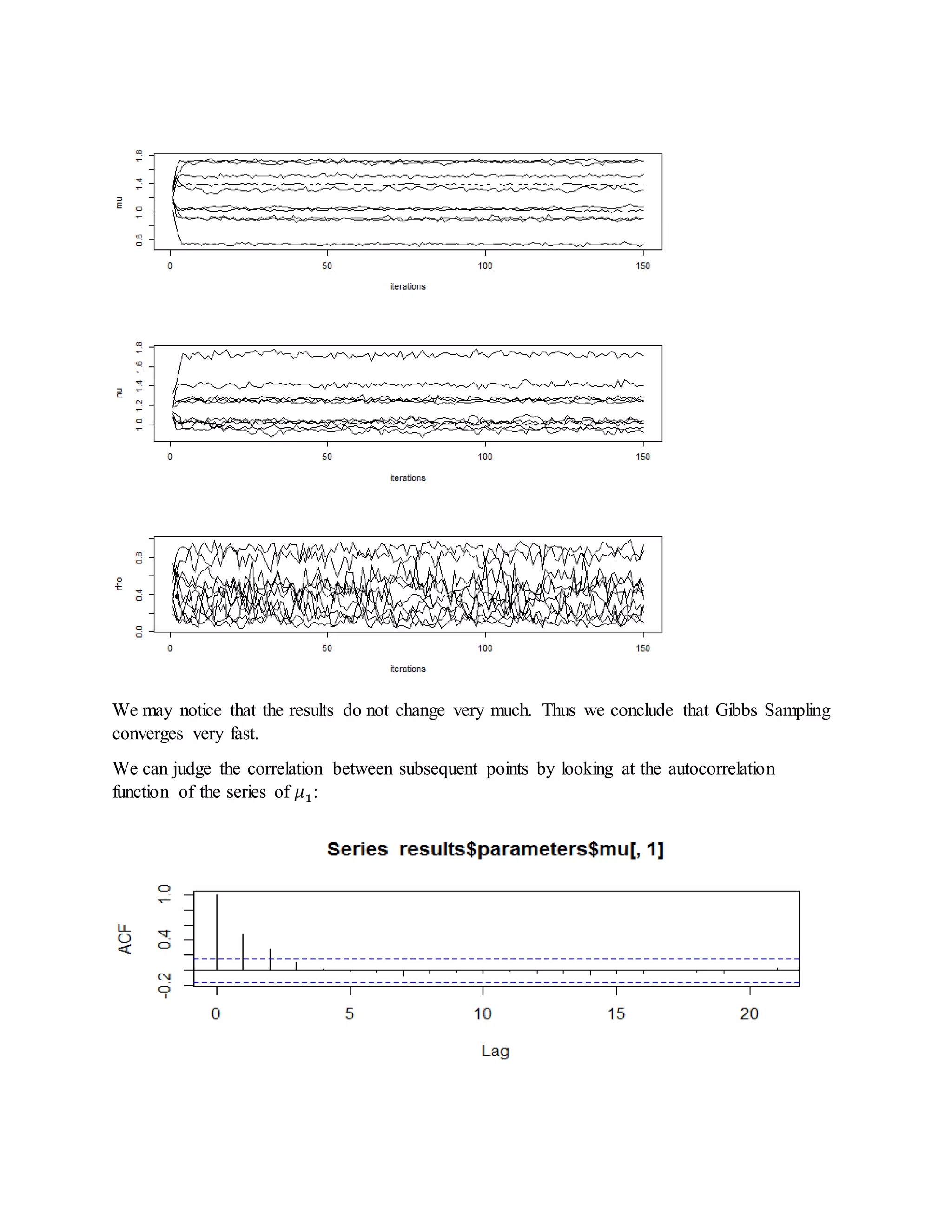- It also derives steps for Gibbs sampling to estimate the missing species indicators and parameter values based on their posterior distributions.

1. Maximum Likelihood Estimation of Beetle’s Species from Its Mass,
Length and Other Characters
LIANGKAI HU
1. Derivation of the EM steps
The likelihood of the whole data set is (suppose we know all the missing species
information):
𝐿( 𝜇, 𝜈, 𝜌, 𝛼) = ∏ 𝑃( 𝑚 𝑖, 𝑟𝑖, 𝑠𝑖| 𝑠𝑝𝑖) ∙ 𝑃(𝑠𝑝𝑖)
𝑁
𝑖=1
= ∏
1
0.08√2𝜋
∙ exp{−
( 𝑙𝑜𝑔 𝑚 𝑖 − 𝜇 𝑠)2
2 ∙ 0.082
}
𝑁
𝑖=1
∙
1
0.1 ∙ √2𝜋
∙ exp{−
(𝑙𝑜𝑔 𝑟𝑖 − 𝜈𝑠 )2
2 ∙ 0.12
} ∙ 𝜌𝑠
𝑠𝑖
(1 − 𝜌𝑠)1−𝑠𝑖 ∙ 𝛼 𝑠𝑝
𝑙( 𝜇, 𝜈, 𝜌, 𝛼) = ∑ log(
1
0.008 ∙ 2𝜋
) −
( 𝑙𝑜𝑔 𝑚 𝑖 − 𝜇 𝑠)2
2 ∙ 0.082
−
( 𝑙𝑜𝑔 𝑚 𝑖 − 𝜇 𝑠)2
2 ∙ 0.082
+ 𝑠𝑖 log 𝜌𝑠
𝑁
𝑖=1
+(1 − 𝑠𝑖)log(1 − 𝜌𝑠 ) + log 𝛼 𝑠
However, we have some observations whose species are not known, while others
whose species are not known, but genus are known. Thus we need to divide the data
into three groups U, V, W as follows:
𝑈 = { 𝑜𝑏𝑠. 𝑖: 𝑤ℎ𝑜𝑠𝑒 𝑒𝑥𝑎𝑐𝑡 𝑠𝑝𝑒𝑐𝑖𝑒𝑠 𝑎𝑟𝑒 𝑘𝑛𝑜𝑤𝑛}
𝑉 = { 𝑜𝑏𝑠. 𝑖: 𝑤ℎ𝑜𝑠𝑒 𝑠𝑝𝑒𝑐𝑖𝑒𝑠 𝑎𝑟𝑒 𝑛𝑜𝑡 𝑘𝑛𝑜𝑤𝑛 𝑏𝑢𝑡 𝑔𝑒𝑛𝑢𝑠 𝑎𝑟𝑒 𝑘𝑛𝑜𝑤𝑛}
𝑊 = { 𝑜𝑏𝑠. 𝑖: 𝑛𝑒𝑖𝑡ℎ𝑒𝑟 𝑠𝑝𝑒𝑐𝑖𝑒𝑠 𝑛𝑜𝑟 𝑔𝑒𝑛𝑢𝑠 𝑎𝑟𝑒 𝑘𝑛𝑜𝑤𝑛}
E step: We want to find the distribution of the missing data Z (i.e. species for some
observations) given all the known information.
We denote the probability that obs. i is actually species j as 𝑃𝑖𝑗. Note that {𝑃𝑖𝑗} is a
500𝑥10 matrix.
○1 For obs. 𝑖 in U, 𝑃𝑖𝑗 = 1 𝑓𝑜𝑟 𝑗 = 𝑡ℎ𝑒 𝑘𝑛𝑜𝑤𝑛 𝑠𝑝𝑒𝑐𝑖𝑒𝑠 𝑜𝑓 𝑜𝑏𝑠. 𝑖, 𝑃𝑖𝑗 = 0 𝑜. 𝑤.
○2 For obs. in V:
Note, for example, if some obs. i is of genus 1, then j can only be 1,2,3, so
𝑃𝑖1 + 𝑃𝑖2 + 𝑃𝑖3 = 1 and 𝑃𝑖𝑗 = 0 for 𝑗 = 4, …,10. Then we have
𝑃𝑖𝑗 = 𝑃{𝑍𝑖 = 𝑗|𝑚 𝑖, 𝑟𝑖, 𝑠𝑖, 𝜃( 𝑡)
} =
𝑃(𝑚 𝑖, 𝑟𝑖, 𝑠𝑖|𝑧𝑖 = 𝑗, 𝜃( 𝑡)
) ∙ 𝑃(𝑍𝑖 = 𝑗|𝜃( 𝑡)
)
∑ 𝑃(𝑚 𝑖, 𝑟𝑖, 𝑠𝑖|𝑍𝑖 = 𝑟,𝑟∈𝐺(𝑖) 𝜃( 𝑡)
) ∙ 𝑃(𝑍𝑖 = 𝑟|𝜃( 𝑡)
)

2. 𝐺(𝑖) means all the possible species that obs. i can be. For example, if genus of some
obs. i is known to be 1, then 𝐺( 𝑖) = {1,2,3}.
Notice that 𝑃(𝑍𝑖 = 𝑗|𝜃( 𝑡)
) = 𝛼𝑗
( 𝑡)
and
𝑃(𝑚 𝑖, 𝑟𝑖, 𝑠𝑖|𝑧𝑖 = 𝑗, 𝜃( 𝑡)
)
=
1
0.08√2𝜋
∙ exp{−
(𝑙𝑜𝑔 𝑚 𝑖 − 𝜇𝑗
( 𝑡)
)
2
2 ∙ 0.082
} ∙
1
0.1 ∙ √2𝜋
∙ exp{−
(𝑙𝑜𝑔 𝑟𝑖 − 𝜈𝑗
( 𝑡)
)2
2 ∙ 0.12
} ∙ 𝜌𝑗
( 𝑡) 𝑠𝑖
(1 − 𝜌𝑗
( 𝑡)
)
1−𝑠𝑖
○3 For obs. in W:
Since no species information are known about these observations, so j can range from
1 to 10 for every obs.
𝑃𝑖𝑗 =
𝑃(𝑚 𝑖, 𝑟𝑖, 𝑠𝑖|𝑍𝑖 = 𝑗, 𝜃( 𝑡)
) ∙ 𝑃(𝑍𝑖 = 𝑗|𝜃( 𝑡)
)
∑ 𝑃(𝑚 𝑖, 𝑟𝑖, 𝑠𝑖|𝑍𝑖 = 𝑟, 𝜃( 𝑡)
) ∙ 𝑃(𝑍𝑖 = 𝑟|𝜃( 𝑡)
)10
𝑟=1
Next we will find the expectation of the log likelihood w.r.t Z. Denote the log
likelihood function of obs. i as 𝑙 𝑖(𝜇 𝑠, 𝜈𝑠 , 𝜌𝑠 , 𝛼 𝑠)where s is the possible species of i.
𝐸 𝑍(𝑙|𝜃( 𝑡)
) = ∑ ∑ 𝑃𝑖𝑗 ∙ 𝑙 𝑖(𝜇 𝑗, 𝜈𝑗, 𝜌𝑗 , 𝛼𝑗)
10
𝑗=1
500
𝑖=1
M Step:
In M step, we want to find 𝜇, 𝜈, 𝜌, 𝛼 such that 𝐸 𝑍𝑖
(𝑙(𝜇, 𝜈, 𝜌, 𝛼)|𝜃( 𝑡)
) is maximized.
To achieve this, we take partial derivatives of 𝐸 𝑍𝑖
(𝑙(𝜇, 𝜈, 𝜌, 𝛼)|𝜃( 𝑡)
) w.r.t. each
parameters and set them to zero. We get:
1) For 𝜇 𝑠:
𝜕𝐸( 𝑙)
𝜕 𝜇 𝑠
= ∑ 𝑃𝑖𝑠
log 𝑚𝑖−𝜇 𝑠
0.082
500
𝑖=1
2) For 𝜈𝑠 : (Similar as above)
3) For 𝜌𝑠 :
𝜕𝐸( 𝑙)
𝜕 𝜇 𝑠
=
1
𝜌 𝑠
(∑ 𝑃𝑖𝑠 ∙ 𝑠𝑖
500
𝑖=1 ) +
1
1−𝜌 𝑠
(∑ 𝑃𝑖𝑠 ∙500
𝑖=1 (1 − 𝑠𝑖))
By solving these equations, we get the following result:
𝜇 𝑠 =
∑ 𝑃𝑖𝑠 ∙ log 𝑚𝑖𝑖
∑ 𝑃𝑖𝑠𝑖

3. 𝜈𝑠 =
∑ 𝑃𝑖𝑠 ∙ log 𝑟𝑖𝑖
∑ 𝑃𝑖𝑠𝑖
𝜌𝑠 =
∑ 𝑃𝑖𝑠 ∙ 𝑠𝑖𝑖
∑ 𝑃𝑖𝑠𝑖
To find 𝛼 𝑠, we need to solve the following problem:
max ∑ ∑Pis ∙ log 𝛼 𝑠
500
𝑖=1
10
𝑠=1
𝑠𝑢𝑏𝑗𝑒𝑐𝑡 𝑡𝑜 ∑ 𝛼 𝑟
10
𝑟=1
= 1
Lagrange multiplier was used to solve this optimization problem.
The Lagrange equation is:
𝐿( 𝛼, 𝜆) = ∑ ∑ Pis ∙ log 𝛼 𝑠
500
𝑖=1
10
𝑠 =1
+ 𝜆 ∙ (∑ 𝛼 𝑟
10
𝑟=1
− 1)
Set its first order derivative to zero, and we get:
𝜕𝐿
𝜕𝛼 𝑠
= ∑
𝑃𝑖𝑠
𝛼 𝑠
500
𝑖=1 = −𝜆 𝑓𝑜𝑟 𝑠 = 1,… ,10
𝜕𝐿
𝜕𝜆
= ∑ 𝛼 𝑠
10
𝑖=1
= 1
Solving the equations above, we get the final result:
𝛼 𝑠 =
∑ 𝑃𝑖𝑠
500
𝑖=1
𝑁
Finally, the log likelihood function of the observed data is:
𝑙( 𝜇, 𝜈, 𝜌, 𝛼) = ∑ log (∑ 𝐿 𝑖(𝜇𝑗, 𝜈𝑗, 𝜌𝑗 , 𝛼𝑗)
𝑗
)
500
𝑖=1
Here for each 𝑖, 𝑗 belongs to the set of all the possible species of obs. 𝑖.

4. 2. Results and discussion
After running 120 iterations, the result become stable within a small interval.
Species mu nu rho alpha
1 0.89429230531416382 1.03426438306816149 0.265733858674903622 0.067298939652255960
2 1.38996762809172703 0.96230142865978008 0.099347396713654113 0.194401480749592737
3 1.71685888287966826 1.05462477433474833 0.155178243458189369 0.076713456308002470
4 0.53124009522079751 1.26205166839992011 0.817691807359486988 0.073477794818745140
5 1.50946001386076034 1.40867770953983351 0.918358415865703770 0.055110000451895985
6 1.72333687565397997 0.99940488257136595 0.146446373184280970 0.105822215585868865
7 1.32082385152815229 0.93800398966601317 0.429516035555412845 0.043668802805622346
8 1.05193497565973648 1.25530539642827943 0.440694262394571323 0.157577787120826457
9 1.02392291475561303 1.23667032047351566 0.460623206492330128 0.192135243325587707
10 0.90466366880025695 1.73042299432002511 0.532830415964590243 0.033794279181602327
The log likelihood is -122.12229914568172. (Please see the output page for the log
likelihood after each iteration.)
The plot of the data and the MLE of these parameters is shown in the graph below:

5. In this plot, ratios are plotted against masses, with the variable swamp represented by two
different signs. The vertical and horizontal lines represent the MLE estimators of 𝜇 and 𝜈,
respectively, of various species. We may tell from the graph that the MLE we have found fit the
data well, as the points are much denser around the lines.
It took 120 steps for the MLE to have 14 digits’ precision. We also want to look at the rate of
convergence of the log likelihood in order to make a thorough conclusion.
For the log likelihood at Step 110,111,112, we have:
Final log likelihood: -122.12229914568185
At Step 100: -122.12229914572499
At Step 101: -122.12229914571668
At Step 102: -122.1222991457101
(P110- final)/(P111-final)= 1.228583029
(P111- final)/(P112-final)= 1.206761391
Thus we conclude the rate of convergence of the log likelihood is approximately 1.
3. Derivation of Gibbs Sampling steps.
Step 1: Update unknown species indicators
As in Assignment 2, denote the probability that obs. i is actually species j as 𝑃𝑖𝑗. Note
that {𝑃𝑖𝑗} is a 500𝑥10 matrix.
Then the species indicator of an observation 𝑖 is a multinomial distribution, with
probabilities indicated by 𝑃𝑖𝑗, 𝑗 = 1 …10. We can use the sample function in R to
generate simulation of species indicator.
Step 2: Obtain a sample of parameters based on their posterior distribution
The posterior probability of parameters is:
𝑃(𝜇, 𝜈, 𝜌|𝑋, 𝑌, 𝑍, 𝜃( 𝑡)
) ∝ 𝑃( 𝜇) ∙ ∏ 𝑃( 𝑋𝑖| 𝜇) ∙ 𝑃( 𝜈) ∙ ∏ 𝑃( 𝑌𝑖| 𝜈) ∙ 𝑃( 𝜌) ∙ ∏ 𝑃(𝑍𝑖|𝜌𝑠 )
𝑁
𝑖=1
𝑁
𝑖=1
𝑁
𝑖=1
𝑤ℎ𝑒𝑟𝑒
𝜇 = ( 𝜇1,… , 𝜇10) 𝜈 = ( 𝜈1, … , 𝜈10) 𝜌 = (𝜌1, … , 𝜌10)
𝑋𝑖 = log 𝑚𝑎𝑠𝑠 𝑜𝑓 𝑜𝑏𝑠. 𝑖 𝑌𝑖 = log 𝑟𝑎𝑡𝑖𝑜 𝑜𝑓 𝑜𝑏𝑠. 𝑖 𝑍𝑖 = 𝑠𝑤𝑎𝑚𝑝 𝑖𝑛𝑑𝑖𝑐𝑎𝑡𝑜𝑟 𝑜𝑓 𝑜𝑏𝑠. 𝑖
Then for some 𝑠, we have

6. 𝑃( 𝜇 𝑠|𝑋) ∝ exp(−
1
2
∙
( 𝜇 𝑠 − 1)2
22
) ∙ ∏ exp(−
1
2
∙
( 𝑋𝑖 − 𝜇 𝑠)2
0.082
)
{ 𝑖:𝑠𝑝𝑒𝑐𝑖𝑒𝑠( 𝑖)=𝑠}
We want that 𝑃( 𝜇 𝑠|𝑋) to have the form exp(−
1
2
( 𝜇 𝑠−𝑚)2
𝑠2 ). After expansion and comparison, we
get
𝑚 =
1
22 ∙ 1 +
𝑛 𝑠
0.082 ∙ 𝑋𝑠
̅̅̅
1
22 +
𝑛 𝑠
0.082
𝑠2
= (
1
22
+
𝑛 𝑠
0.082
)
−1
Thus 𝜇 𝑠|𝑋~𝑁𝑜𝑟𝑚𝑎𝑙 (𝑚, 𝑠2
).
Similarly,
𝑃( 𝜈𝑠|𝑋) ∝ exp(−
1
2
∙
( 𝜈𝑠 − 1)2
22
) ∙ ∏ exp(−
1
2
∙
( 𝑋𝑖 − 𝜈𝑠 )2
0.102
)
{ 𝑖:𝑠𝑝𝑒𝑐𝑖𝑒𝑠 ( 𝑖)=𝑠}
𝜈𝑠 |𝑋~𝑁𝑜𝑟𝑚𝑎𝑙 (𝑚, 𝑠2
)
𝑤ℎ𝑒𝑟𝑒
𝑚 =
1
22 ∙ 1 +
𝑛 𝑠
0.102 ∙ 𝑌𝑠
̅
1
22 +
𝑛 𝑠
0.102
𝑠2
= (
1
22
+
𝑛 𝑠
0.102
)
−1
Finally, we have
𝑃( 𝜌𝑠 | 𝑍) ∝
1
1 − 0
∙ ∏ 𝜌𝑠
𝑍𝑖 ∙ (1 − 𝜌𝑠)1−𝑍𝑖
{ 𝑖:𝑠𝑝𝑒𝑐𝑖𝑒𝑠( 𝑖)=𝑠}
∝ 𝜌𝑠
(∑ 𝑍𝑖 +1)−1
∙ (1 − 𝜌𝑠)(𝑛 𝑠−∑ 𝑍𝑖 +1)−1
Thus 𝜌𝑠 |𝑍~𝐵𝑒𝑡𝑎(∑ 𝑍𝑖 + 1, 𝑛 𝑠 + 1 − ∑ 𝑍𝑖)
4. Results and discussions
Initial points are chosen in the same fashion as we did in Assignment 2, i.e. we set them
to their corresponding means of data, regardless of species. The result is as below:

7. After looking at the graphs, we decide to set the first 20 iterations as burn-in. We get the mean and
standard deviation of the parameters:
𝜇
Gibbs sampling of all parameters

8. 𝜈
𝜌
The followings are two plots of the simulated species indicators for observation No. 3 (genus
known as 4) and No. 8 (genus unknown).
From the plots of 𝜇 and 𝜈, we can determine that it takes only about 10 steps for Gibbs sampling
to converge to the true distribution. If we set initial points farther away from the true value, we
get results like below (in this case all 𝜇′𝑠 are set to 2, 𝜈′𝑠 to 2 and 𝜌′𝑠 to 0.5):
Simulated species indicators for obs. 3 and 8
Gibbs Sampling for parameters (initialpoints set far awayfrom true values)

9. We may notice that the results do not change very much. Thus we conclude that Gibbs Sampling
converges very fast.
We can judge the correlation between subsequent points by looking at the autocorrelation
function of the series of 𝜇1:

10. From this graph, we can tell that the autocorrelation at lag 1 and 2 are significant. This is a little
different from what we would expect from generating a series using Markov chain, as the current
state is only dependent on the last state.