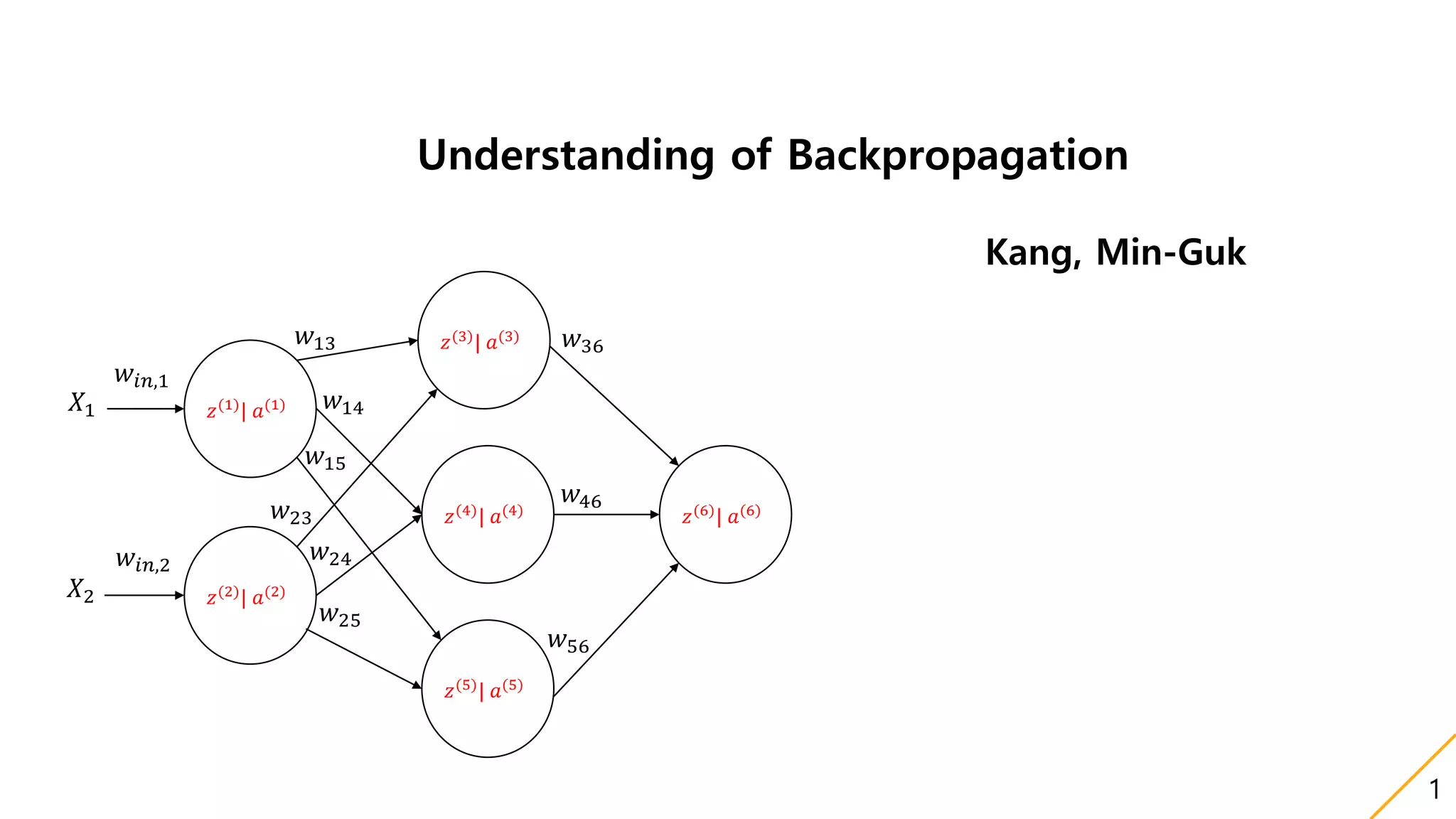
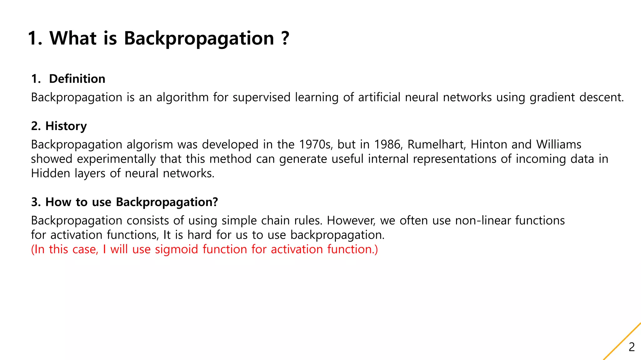
This document discusses backpropagation, an algorithm for supervised learning of artificial neural networks using gradient descent. It provides definitions and history of backpropagation, and explains how to use it with three main points: 1) It uses simple chain rules to calculate derivatives between weights in different layers to update weights. 2) Preparations include defining a cost function and the derivative of the sigmoid activation function commonly used. 3) The weight updates are dependent on derivatives from previous layers, and both forward and backward paths must be considered to calculate some derivatives between weights. Gradient descent is then applied to renew the weights.

1. Understanding of Backpropagation
Kang, Min-Guk
𝑋1
𝑋2
𝑧(1)
| 𝑎(1)
𝑧(2)
| 𝑎(2)
𝑧(3)
| 𝑎(3)
𝑧(4)
| 𝑎(4)
𝑧(5)
| 𝑎(5)
𝑧(6)
| 𝑎(6)
𝑤13 𝑤36
𝑤14
𝑤15
𝑤23
𝑤24
𝑤25
𝑤46
𝑤56
𝑤𝑖𝑛,1
𝑤𝑖𝑛,2
1

2. 1. What is Backpropagation ?
1. Definition
Backpropagation is an algorithm for supervised learning of artificial neural networks using gradient descent.
2. History
Backpropagation algorism was developed in the 1970s, but in 1986, Rumelhart, Hinton and Williams
showed experimentally that this method can generate useful internal representations of incoming data in
Hidden layers of neural networks.
3. How to use Backpropagation?
Backpropagation consists of using simple chain rules. However, we often use non-linear functions
for activation functions, It is hard for us to use backpropagation.
(In this case, I will use sigmoid function for activation function.)
2

3. 2. Preparations
1. Cost function(Loss function)
I will use below cost function(𝑦𝑎 is value of hypothesis, 𝑦𝑡 is value of true)
𝐶 =
1
2
(𝑦𝑎 − 𝑦𝑡)2
2. Derivative of sigmoid function
𝑑𝑆(𝑧)
𝑑𝑧
=
1
(1+𝑒−𝑧)2 × −1 × −𝑒−𝑧 = 𝑆(𝑧)(1 − 𝑆(𝑧))
∵ Sigmoid function = S(z) =
1
1+𝑒−𝑧 , 𝐹 𝑧 =(
1
𝑔 𝑧
) =
− 𝑔 𝑧
𝑔 𝑧 2
3. How to renew weights using Gradient descent
𝑊𝑖→𝑗,𝑛𝑒𝑤 = 𝑊𝑖→𝑗,𝑜𝑙𝑑 − η
𝜕𝐶
𝜕𝑊 𝑖→𝑗,𝑜𝑙𝑑
(η is learning rate)
3

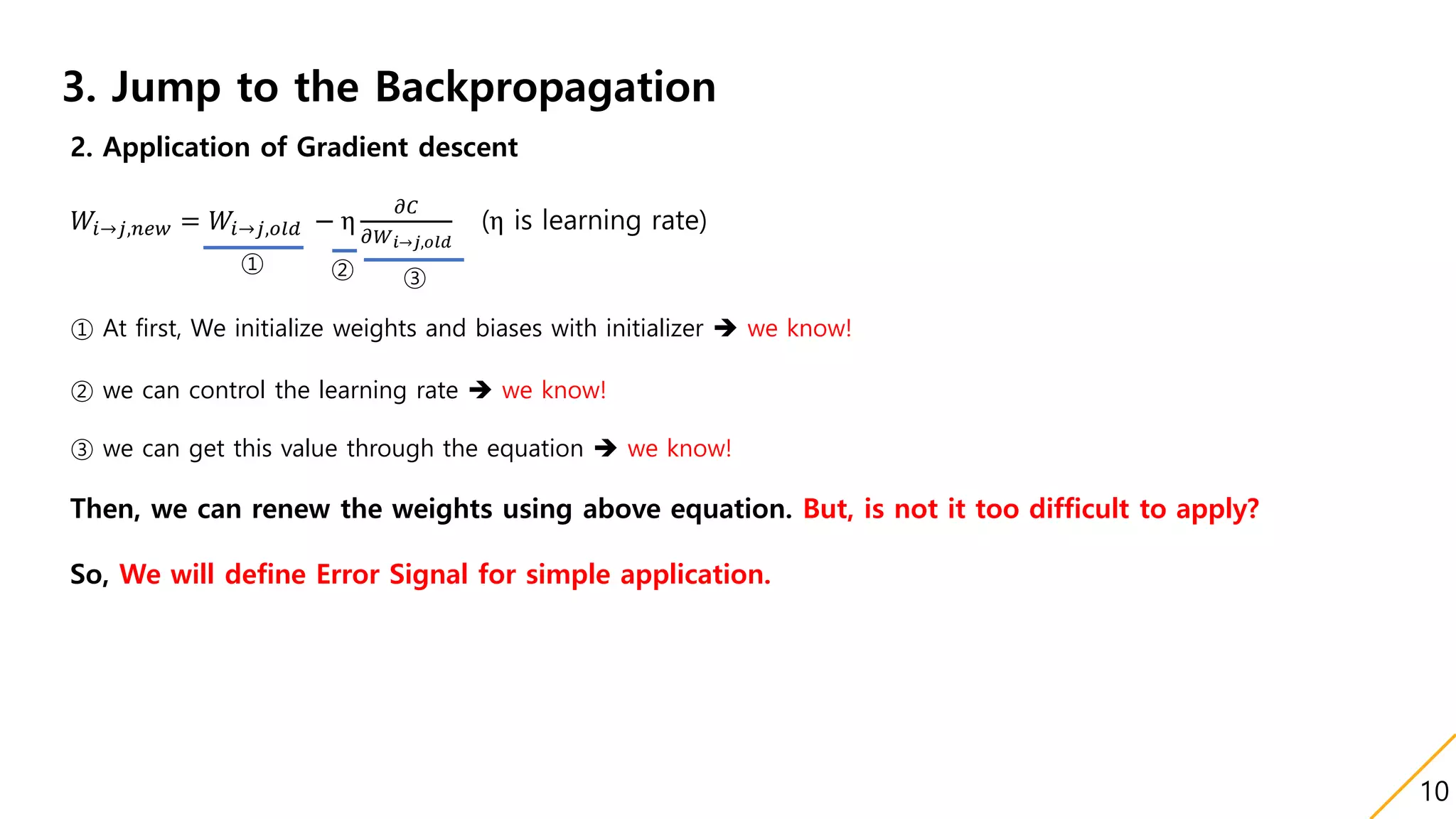
4. 3. Jump to the Backpropagation
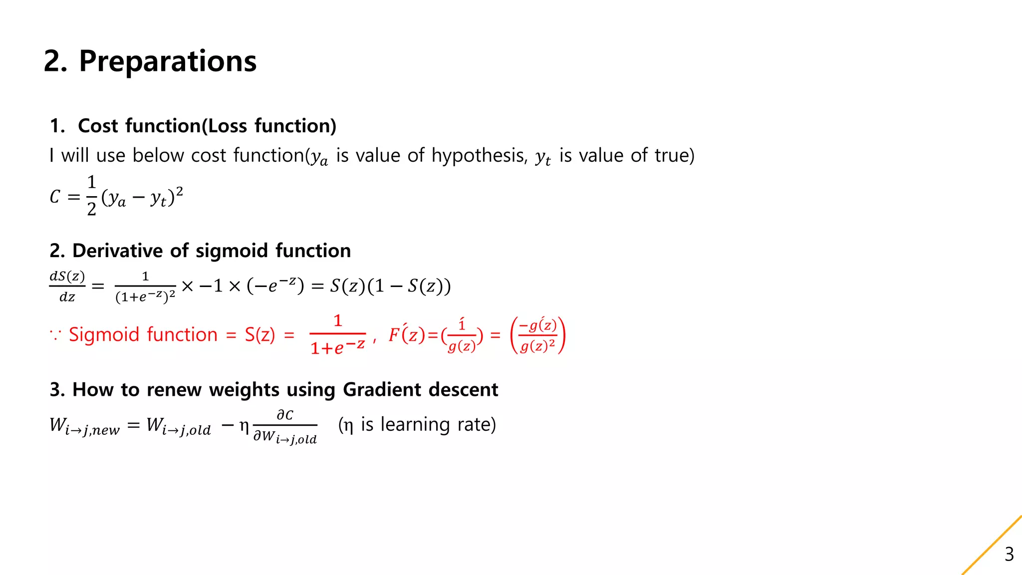
1. Derivative Relationship between weights
1-1. The weight update is dependent on derivatives that reside previous layers.(The Word previous means it is located right side )
𝐶 =
1
2
(𝑦𝑎 − 𝑦𝑡)2
→
𝜕𝐶
𝜕𝑊2,3
= (𝑦𝑎 − 𝑦𝑡) ×
𝜕𝑦 𝑎
𝜕𝑊2,3
= (𝑦𝑎 − 𝑦𝑡) ×
𝜕
𝜕𝑊2,3
[σ{𝑧(3)
}] (σ is sigmoid function)
𝜕𝐶
𝜕𝑊2,3
= (𝑦𝑎 − 𝑦𝑡) ×σ{𝑧(3)
} × [1 − σ{𝑧(3)
}] ×
𝜕𝑍3
𝜕𝑊2,3
= (𝑦𝑎 − 𝑦𝑡) ×σ{𝑧(3)
} × [1 − σ{𝑧(3)
}] ×
𝜕
𝜕𝑊2,3
( 𝑎(2)
𝑤2,3)
∴
𝜕𝐶
𝜕𝑊2,3
= (𝑦𝑎 − 𝑦𝑡)σ{𝑧(3)
}[1 − σ{𝑧(3)
}] 𝑎(2)
1𝑋𝑖𝑛 2 3
𝑤1,2 𝑤2,3
𝑤𝑖𝑛,1
𝑧(2)
| 𝑎(2)
𝑧(1)
| 𝑎(1)
𝑧(3)
| 𝑎(3)
𝑎(3)
= 𝑦𝑎
Feed forward
Backpropagation
4

5. 3. Jump to the Backpropagation
1. Derivative Relationship between weights
1-1. The weight update is dependent on derivatives that reside previous layers.(The Word previous means it is located right side )
𝐶 =
1
2
(𝑦𝑎 − 𝑦𝑡)2
→
𝜕𝐶
𝜕𝑊1,2
= (𝑦𝑎 − 𝑦𝑡) ×
𝜕𝑦 𝑎
𝜕𝑊1,2
= (𝑦𝑎 − 𝑦𝑡) ×
𝜕
𝜕𝑊1,2
[σ{𝑧(3)
}] (σ is sigmoid function)
𝜕𝐶
𝜕𝑊1,2
= (𝑦𝑎 − 𝑦𝑡) ×σ{𝑧(3)
} × [1 − σ{𝑧(3)
}] ×
𝜕𝑍3
𝜕𝑊1,2
= (𝑦𝑎 − 𝑦𝑡) ×σ{𝑧(3)
} × [1 − σ{𝑧(3)
}] ×
𝜕
𝜕𝑊1,2
( 𝑎(2)
𝑤2,3)
𝜕𝐶
𝜕𝑊1,2
= (𝑦𝑎 − 𝑦𝑡) ×σ{𝑧(3)
} × [1 − σ{𝑧(3)
}] × 𝑤2,3 ×
𝜕
𝜕𝑊1,2
𝑎(2)
= (𝑦𝑎 − 𝑦𝑡) ×σ{𝑧(3)
} × [1 − σ{𝑧(3)
}] × 𝑤2,3 ×
𝜕
𝜕𝑊1,2
σ{𝑧(2)
}
∴
𝜕𝐶
𝜕𝑊1,2
= (𝑦𝑎 − 𝑦𝑡)σ{𝑧(3)
}[1 − σ{𝑧(3)
}] 𝑤2,3 σ{𝑧(2)
}[1 − σ{𝑧(2)
} ] 𝑎(1)
1𝑋𝑖𝑛 2 3
𝑤1,2 𝑤2,3
𝑤𝑖𝑛,1
𝑧(2)
| 𝑎(2)
𝑧(1)
| 𝑎(1)
𝑧(3)
| 𝑎(3)
𝑎(3)
= 𝑦𝑎
Feed forward
Backpropagation
5

6. 3. Jump to the Backpropagation
1. Derivative Relationship between weights
1-1. The weight update is dependent on derivatives that reside previous layers.(The Word previous means it is located right side )
𝐶 =
1
2
(𝑦𝑎 − 𝑦𝑡)2
→
𝜕𝐶
𝜕𝑊 𝑖𝑛,1
= (𝑦𝑎 − 𝑦𝑡) ×
𝜕𝑦 𝑎
𝜕𝑊 𝑖𝑛,1
= (𝑦𝑎 − 𝑦𝑡) ×
𝜕
𝜕𝑊 𝑖𝑛,1
[σ{𝑧(3)
}] (σ is sigmoid function)
Using same way, we will get below equation.
𝜕𝐶
𝜕𝑊 𝑖𝑛,1
= (𝑦𝑎 − 𝑦𝑡)σ{𝑧(3)
}[1 − σ{𝑧(3)
}] 𝑤2,3 σ{𝑧(2)
}[1 − σ{𝑧(2)
} ] 𝑤1,2 σ{𝑧(1)
}[1 − σ{𝑧(1)
} ] 𝑋𝑖𝑛
1𝑋𝑖𝑛 2 3
𝑤1,2 𝑤2,3
𝑤𝑖𝑛,1
𝑧(2)
| 𝑎(2)
𝑧(1)
| 𝑎(1)
𝑧(3)
| 𝑎(3)
𝑎(3)
= 𝑦𝑎
Feed forward
Backpropagation
6

7. 3. Jump to the Backpropagation
1. Derivative Relationship between weights
1-2. The weight update is dependent on derivatives that reside on both paths.
To get the result, you have to do more tedious calculations than the previous one. So I now just write the result of it.
If you want to know the calculation process, look at the next slide!
𝜕𝐶
𝜕𝑊 𝑖𝑛,1
= (𝑦𝑎 − 𝑦𝑡) 𝑋𝑖𝑛[ σ{𝑧(2)
}[1 − σ{𝑧(2)
}]𝑤2,4 σ{𝑧(1)
}[1 − σ{𝑧(1)
}] 𝑤1,2 + σ{𝑧(3)
}[1 − σ{𝑧(3)
}]𝑤3,4 σ{𝑧(1)
}[1 − σ{𝑧(1)
}]𝑤1,3]
① ② ③ ④
2
3
𝑋𝑖𝑛 1
𝑤𝑖𝑛,1
4 𝑎(3) = 𝑦𝑎
Feed forward
𝑧(4)
| 𝑎(4)
𝑧(3)
| 𝑎(3)
𝑧(1)| 𝑎(1)
𝑤1,2 𝑤2,4
𝑤3,4𝑤1,3
𝑧(2)
| 𝑎(2)
①②
③④
7

8. 2
3
𝑋𝑖𝑛 1
𝑤𝑖𝑛,1
4 𝑎(3)
= 𝑦𝑎
Feed forward
𝑧(4)
| 𝑎(4)
𝑧(3)
| 𝑎(3)
𝑧(1)
| 𝑎(1)
𝑤1,2 𝑤2,4
𝑤3,4𝑤1,3
𝑧(2)
| 𝑎(2)
𝜕𝐶
𝜕𝑊 𝑖𝑛,1
=
𝜕
𝜕𝑊 𝑖𝑛,1
1
2
(𝑦𝑎 − 𝑦𝑡)2
= 𝑦𝑎 − 𝑦𝑡 (
𝜕
𝜕𝑊 𝑖𝑛,1
(σ{𝑧 2
}𝑤2,4 + σ{𝑧 3
}𝑤3,4))
𝜕𝐶
𝜕𝑊 𝑖𝑛,1
= 𝑦𝑎 − 𝑦𝑡 [ 𝑤2,4
𝜕
𝜕𝑊 𝑖𝑛,1
σ{𝑧 2
} + 𝑤3,4
𝜕
𝜕𝑊 𝑖𝑛,1
σ{𝑧 3
} ] = 𝑦𝑎 − 𝑦𝑡 [ 𝑤2,4σ{𝑧 2
}
𝜕
𝜕𝑊 𝑖𝑛,1
(σ{𝑧 1
}𝑤1,2)+
𝑤3,4σ{𝑧 3
}
𝜕
𝜕𝑊 𝑖𝑛,1
(σ{𝑧 1
}𝑤1,3) ]
𝜕𝐶
𝜕𝑊 𝑖𝑛,1
= 𝑦𝑎 − 𝑦𝑡 [ 𝑤2,4σ{𝑧 2
}𝑤1,2σ{𝑧 1
}
𝜕
𝜕𝑊 𝑖𝑛,1
(𝑋𝑖𝑛 𝑤𝑖𝑛,1) + 𝑤3,4σ{𝑧 3
} 𝑤1,3 σ{𝑧 1
}
𝜕
𝜕𝑊 𝑖𝑛,1
(𝑋𝑖𝑛 𝑤𝑖𝑛,1) ]
𝜕𝐶
𝜕𝑊 𝑖𝑛,1
= 𝑦𝑎 − 𝑦𝑡 [ 𝑤2,4σ{𝑧 2
}𝑤1,2σ{𝑧 1
} 𝑋𝑖𝑛 + 𝑤3,4σ{𝑧 3
} 𝑤1,3 σ{𝑧 1
}𝑋𝑖𝑛 ]
= (𝑦𝑎 − 𝑦𝑡) 𝑋𝑖𝑛[ σ{𝑧(2)
}[1 − σ{𝑧(2)
}]𝑤2,4 σ{𝑧(1)
}[1 − σ{𝑧(1)
}] 𝑤1,2 + σ{𝑧(3)
}[1 − σ{𝑧(3)
}]𝑤3,4 σ{𝑧(1)
}[1 − σ{𝑧(1)
}]𝑤1,3]
𝑧(1)
𝑧(1)
8

9. 3. Jump to the Backpropagation
1. Derivative Relationship between weights
1-3. The derivative for a weight is not dependent on the derivatives of any of the other weights in the same layer.
This is easy, so I will not explain it here.(homework )
𝑋1
𝑋2
1
2
3
4
5
6
𝑤13 𝑤36
𝑤14
𝑤15
𝑤23
𝑤24
𝑤25
𝑤46
𝑤56
𝑤(1)
𝑤(2)
Independant
9

10. 3. Jump to the Backpropagation
2. Application of Gradient descent
𝑊𝑖→𝑗,𝑛𝑒𝑤 = 𝑊𝑖→𝑗,𝑜𝑙𝑑 − η
𝜕𝐶
𝜕𝑊 𝑖→𝑗,𝑜𝑙𝑑
(η is learning rate)
① At first, We initialize weights and biases with initializer  we know!
② we can control the learning rate  we know!
③ we can get this value through the equation  we know!
Then, we can renew the weights using above equation. But, is not it too difficult to apply?
So, We will define Error Signal for simple application.
① ② ③
10

11. 3. Jump to the Backpropagation
3. Error Signals
1-1 Defintion: δ𝒋 =
𝝏𝑪
𝝏𝒁 𝒋
1-2 General Form of Signals
δj =
𝜕C
𝜕Zj
=
𝜕
𝜕Zj
1
2
(𝑦𝑎 − 𝑦𝑡)2
= (𝑦𝑎 − 𝑦𝑡)
𝜕𝑦 𝑎
𝜕𝑍 𝑗
------- ①
𝜕𝑦 𝑎
𝜕𝑍 𝑗
=
𝜕𝑦 𝑎
𝜕𝑎 𝑗
𝜕𝑎 𝑗
𝜕𝑍 𝑗
=
𝜕𝑦 𝑎
𝜕𝑎 𝑗
× σ(𝑧𝑗) (∵ 𝑎𝑗 = σ(𝑧𝑗))
Because neural network consists of Multiple units, we can think all of the units 𝑘 ∈ 𝑜𝑢𝑡𝑠 𝑗 .
So,
𝜕𝑦 𝑎
𝜕𝑍 𝑗
= σ(𝑧𝑗) 𝑘∈𝑜𝑢𝑡𝑠 𝑗
𝜕𝑦 𝑎
𝜕𝑧 𝑘
𝜕𝑧 𝑘
𝜕𝑎 𝑗
𝜕𝑦 𝑎
𝜕𝑍 𝑗
= σ(𝑧𝑗) 𝑘∈𝑜𝑢𝑡𝑠 𝑗
𝜕𝑦 𝑎
𝜕𝑧 𝑘
𝑤𝑗𝑘 (∵ 𝑧 𝑘 = 𝑤𝑗𝑘 𝑎𝑗)
By above equation ① and δk = (𝑦𝑎 − 𝑦𝑡)
𝜕𝑦 𝑎
𝜕𝑍 𝑘
δj = (𝑦𝑎 − 𝑦𝑡) σ(𝑧𝑗) 𝑘∈𝑜𝑢𝑡𝑠 𝑗
𝜕𝑦 𝑎
𝜕𝑧 𝑘
𝑤𝑗𝑘 = (𝑦𝑎 − 𝑦𝑡)σ(𝑧𝑗) 𝑘∈𝑜𝑢𝑡𝑠 𝑗
δk
(𝑦 𝑎−𝑦𝑡)
𝑤𝑗𝑘
∴ δj= σ(𝑧𝑗) 𝑘∈𝑜𝑢𝑡𝑠 𝑗 δk 𝑤𝑗𝑘 , and for starting, we define δ𝑖𝑛𝑖𝑡𝑖𝑎𝑙 = (𝑦𝑎 − 𝑦𝑡)σ{𝑧(𝑖𝑛𝑖𝑡𝑖𝑎𝑙)
}[1 − σ{𝑧(𝑖𝑛𝑖𝑡𝑖𝑎𝑙)
}]
11

12. 3. Jump to the Backpropagation
3. Error Signals
1-3 The General Form of weight variation
( ※ 𝑊3→6,𝑛𝑒𝑤= 𝑊3→6,𝑜𝑙𝑑 − η
𝜕𝐶
𝜕𝑊3→6,𝑜𝑙𝑑
)
( ※ δ6 = δ𝑖𝑛𝑖𝑡𝑖𝑎𝑙 = (𝑦𝑎 − 𝑦𝑡)σ{𝑧(6)
}[1 − σ{𝑧(6)
}] )
∆𝑊3,6 = −η (𝑦𝑎 − 𝑦𝑡)σ{𝑧(6)
}[1 − σ{𝑧(6)
}] 𝑎(3)
= −ηδ6 𝑎(3)
∆𝑊4,6 = −η (𝑦𝑎 − 𝑦𝑡)σ{𝑧(6)
}[1 − σ{𝑧(6)
}] 𝑎(4)
= −ηδ6 𝑎(4)
∆𝑊5,6 = −η (𝑦𝑎 − 𝑦𝑡)σ{𝑧(6)
}[1 − σ{𝑧(6)
}] 𝑎(5)
= −ηδ6 𝑎(5)
∆𝑊1,3 = −η (𝑦𝑎 − 𝑦𝑡)σ{𝑧(6)
}[1 − σ{𝑧(6)
}] 𝑊3,6 σ{𝑧(3)
}[1 − σ{𝑧(3)
}] 𝑎(1)
= −η ( 𝑘∈𝑜𝑢𝑡𝑠 𝑗 δ6) × 𝑤3,6 σ(𝑧3) 𝑎(1)
= −ηδ3 𝑎(1)
………
∴ ∆𝑊𝑖,𝑗= −ηδ𝑗 𝑎(𝑖)
 We can easily renew weights by using Error Signals δ and Equation ∆𝑾𝒊,𝒋= −𝜼𝜹𝒋 𝒂(𝒊)
𝑋1
𝑋2
𝑧(1)
| 𝑎(1)
𝑧(2)
| 𝑎(2)
𝑧(3)
| 𝑎(3)
𝑧(4)
| 𝑎(4)
𝑧(5)
| 𝑎(5)
𝑧(6)
| 𝑎(6)
𝑤13 𝑤36
𝑤14
𝑤15
𝑤23
𝑤24
𝑤25
𝑤46
𝑤56
𝑤𝑖𝑛,1
𝑤𝑖𝑛,2
12

13. 4. Summarize
Although the picture below is a bit different from my description, Calculations will show you that this is exactly the same as my explanation.
(Picture Source: http://home.agh.edu.pl/~vlsi/AI/backp_t_en/backprop.html) 13

14. 4. Summarize
Although the picture below is a bit different from my description, Calculations will show you that this is exactly the same as my explanation.
(Picture Source: http://home.agh.edu.pl/~vlsi/AI/backp_t_en/backprop.html) 14