The document contains code for several engineering design problems in MATLAB. It includes code to:
1. Design a shaft given inputs of power, rpm, allowable stress, factor of safety, length, and density. It calculates the shaft diameter and weight.
2. Calculate the material saving if a hollow shaft is used instead of a solid shaft, assuming the same input parameters from the first problem.
3. The code demonstrates other engineering design problems can be solved programmatically in MATLAB, such as calculating shape dimensions based on inputs and performing structural analysis calculations.
This slide presents the DDA (Digital Differential Analyzer) algorithm to draw a line between two points, showcasing the code implementation with sample input.
The implementation of Bresenham's line algorithm for drawing a straight line between two specified endpoints is detailed along with the code and input/output examples.
Slides demonstrate code for generating a circle using user-defined center and radius using the Circle Generation Algorithm, showcasing output with input parameters.
A generalized code is shown for performing 2D translation on user-defined points (shapes) with before-and-after plots highlighting transformation details.
This section provides codes for scaling, reflection, and rotation transformations on 2D figures, allowing the user to select transformation types and visualize results.Slides outline a 3D rotation method emphasizing the non-commutative nature of 3D rotations with a code implementation for rotating points about specified axes.
This section introduces a shaft design problem with MATLAB code to calculate the dimensions based on power, speed, shear stress, and safety factor.
MATLAB program is devised to compare material savings between hollow and solid shafts, utilizing parameters such as weight and dimension calculations.
The slide discusses a MATLAB code for designing a cotter joint based on material properties and load requirements, calculating necessary dimensions. This section focuses on selecting deep groove ball bearings based on radial and axial loads, expected life, and inner diameter, with decision-making code.
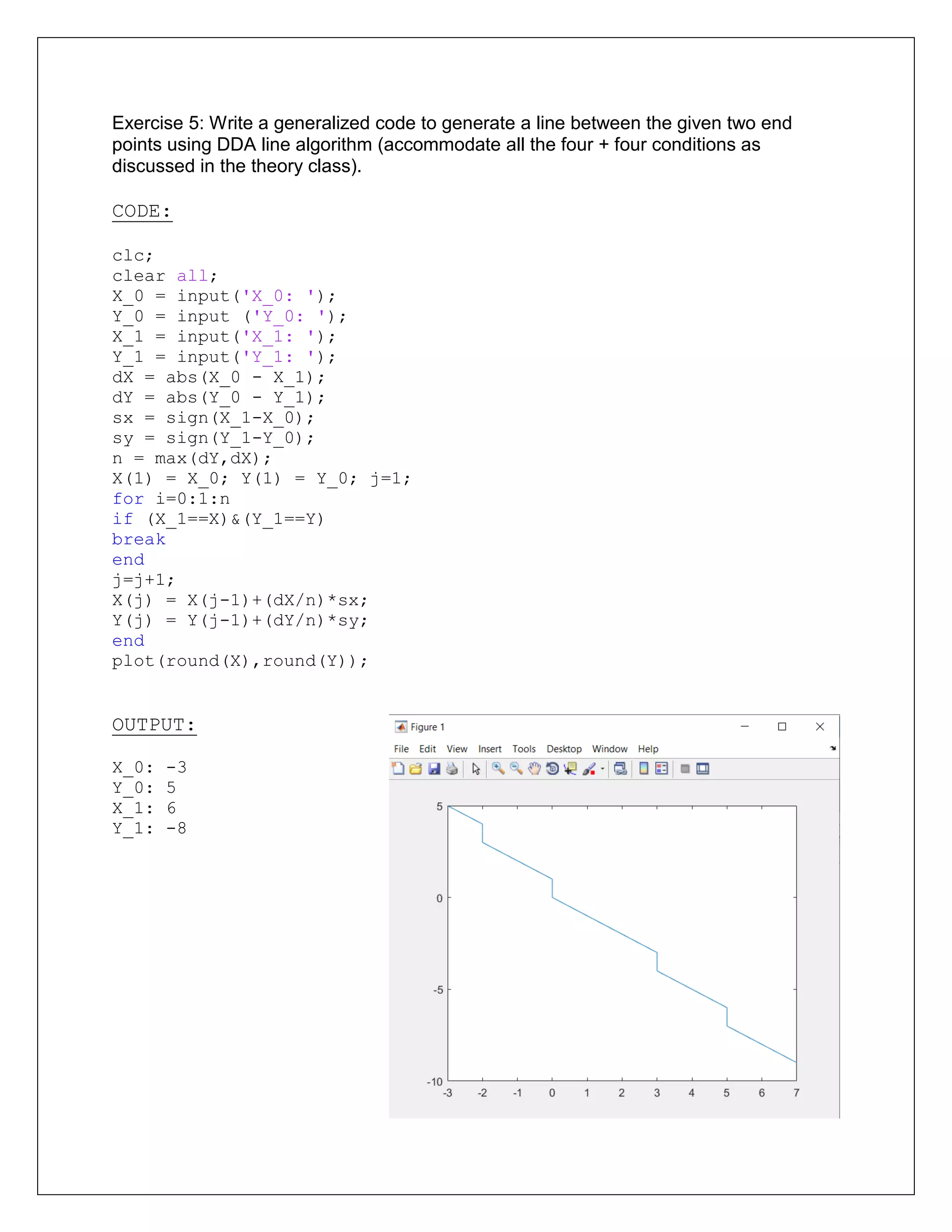
Exercise 5: Writea generalized code to generate a line between the given two end
points using DDA line algorithm (accommodate all the four + four conditions as
discussed in the theory class).
CODE:
clc;
clear all;
X_0 = input('X_0: ');
Y_0 = input ('Y_0: ');
X_1 = input('X_1: ');
Y_1 = input('Y_1: ');
dX = abs(X_0 - X_1);
dY = abs(Y_0 - Y_1);
sx = sign(X_1-X_0);
sy = sign(Y_1-Y_0);
n = max(dY,dX);
X(1) = X_0; Y(1) = Y_0; j=1;
for i=0:1:n
if (X_1==X)&(Y_1==Y)
break
end
j=j+1;
X(j) = X(j-1)+(dX/n)*sx;
Y(j) = Y(j-1)+(dY/n)*sy;
end
plot(round(X),round(Y));
OUTPUT:
X_0: -3
Y_0: 5
X_1: 6
Y_1: -8
3.
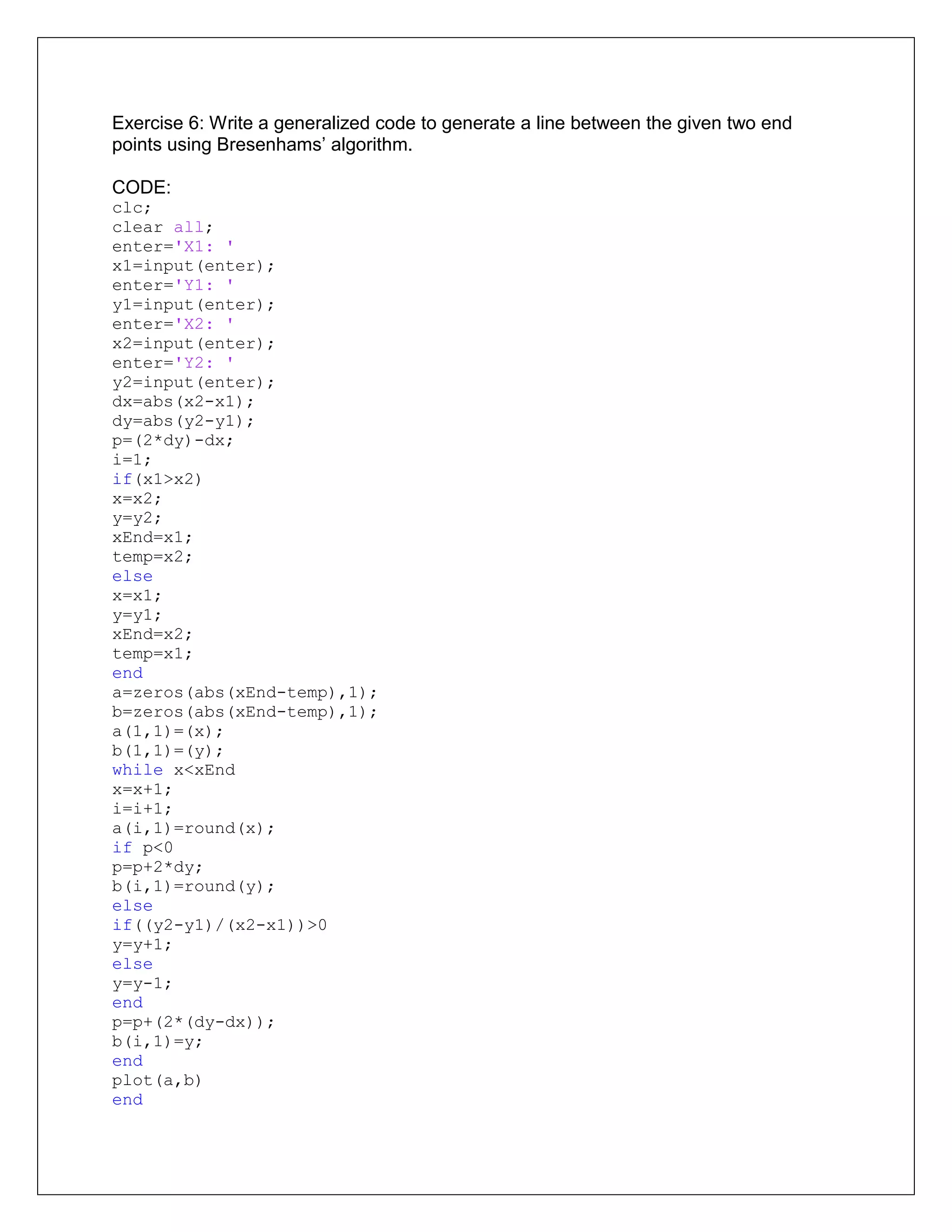
Exercise 6: Writea generalized code to generate a line between the given two end
points using Bresenhams’ algorithm.
CODE:
clc;
clear all;
enter='X1: '
x1=input(enter);
enter='Y1: '
y1=input(enter);
enter='X2: '
x2=input(enter);
enter='Y2: '
y2=input(enter);
dx=abs(x2-x1);
dy=abs(y2-y1);
p=(2*dy)-dx;
i=1;
if(x1>x2)
x=x2;
y=y2;
xEnd=x1;
temp=x2;
else
x=x1;
y=y1;
xEnd=x2;
temp=x1;
end
a=zeros(abs(xEnd-temp),1);
b=zeros(abs(xEnd-temp),1);
a(1,1)=(x);
b(1,1)=(y);
while x<xEnd
x=x+1;
i=i+1;
a(i,1)=round(x);
if p<0
p=p+2*dy;
b(i,1)=round(y);
else
if((y2-y1)/(x2-x1))>0
y=y+1;
else
y=y-1;
end
p=p+(2*(dy-dx));
b(i,1)=y;
end
plot(a,b)
end
4.
OUTPUT:
X1: 2
Y1: 6
X2:9
Y2: 11
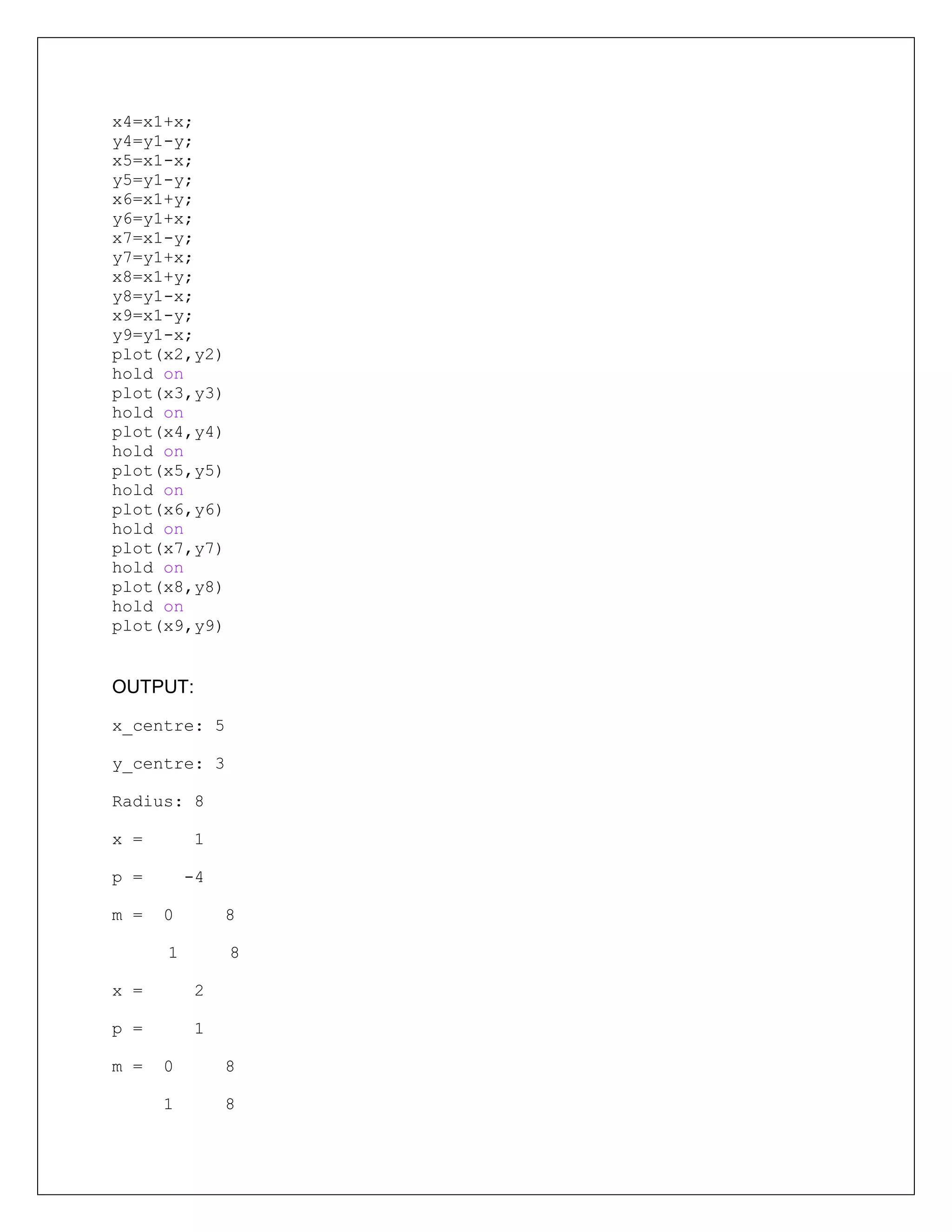
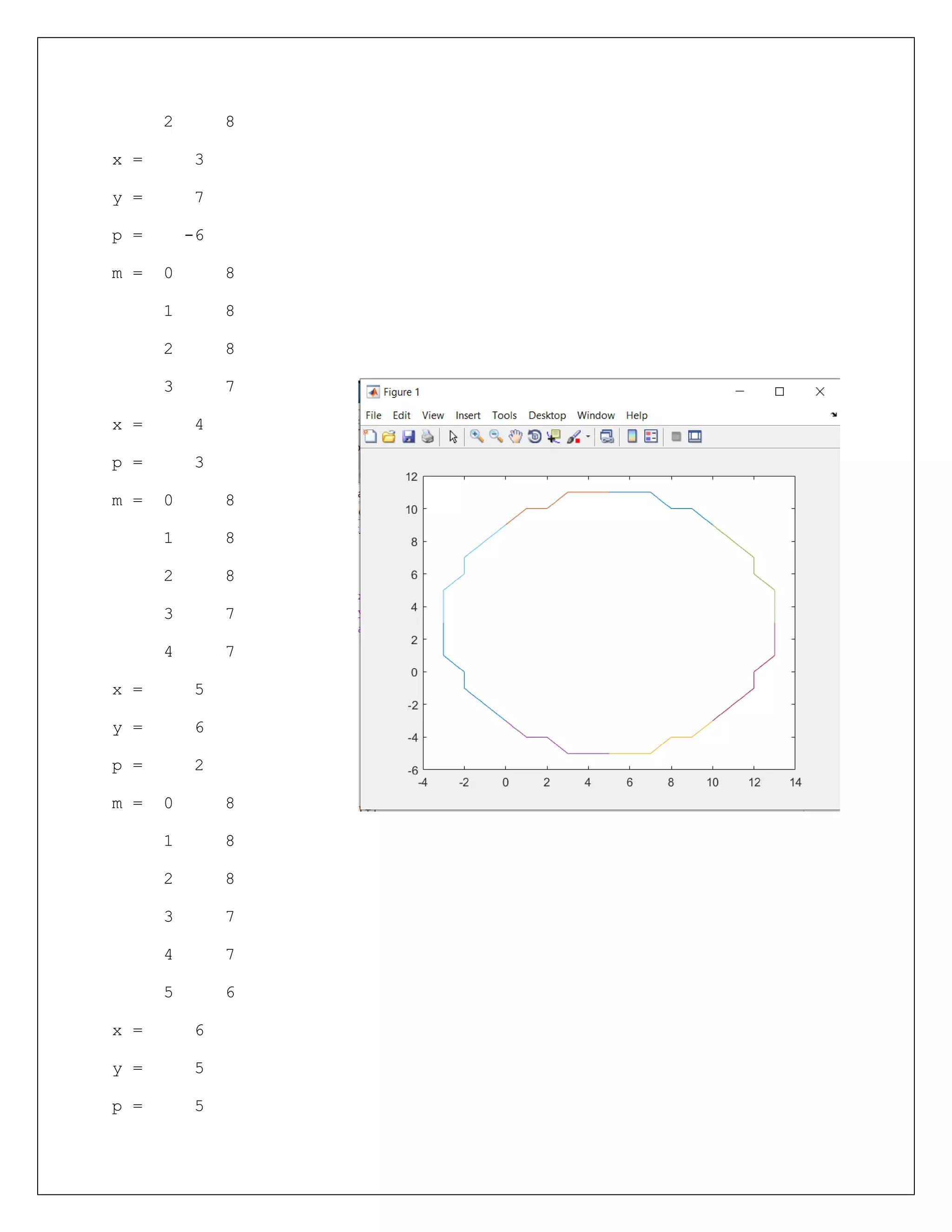
Exercise 7: Write a generalized code to generate a circle for a user specified radius and
coordinates of center point.
CODE:
clc;
clear all;
close all;
x1=input('x_centre: ');
y1=input('y_centre: ');
R=input('Radius: ');
x=0;
y=R;
p=1-R;
m=[x,y];
while(x<y)
x=x+1
if(p<0)
p=p+2*x+1
else
y=y-1
p=p+2*(x-y)+1
end
m=[m;x y]
end
m;
x=m(:,1);
y=m(:,2);
x2=x1+x;
y2=y1+y;
x3=x1-x;
y3=y1+y;
2 8
x =3
y = 7
p = -6
m = 0 8
1 8
2 8
3 7
x = 4
p = 3
m = 0 8
1 8
2 8
3 7
4 7
x = 5
y = 6
p = 2
m = 0 8
1 8
2 8
3 7
4 7
5 6
x = 6
y = 5
p = 5
7.
m = 08
1 8
2 8
3 7
4 7
5 6
6 5
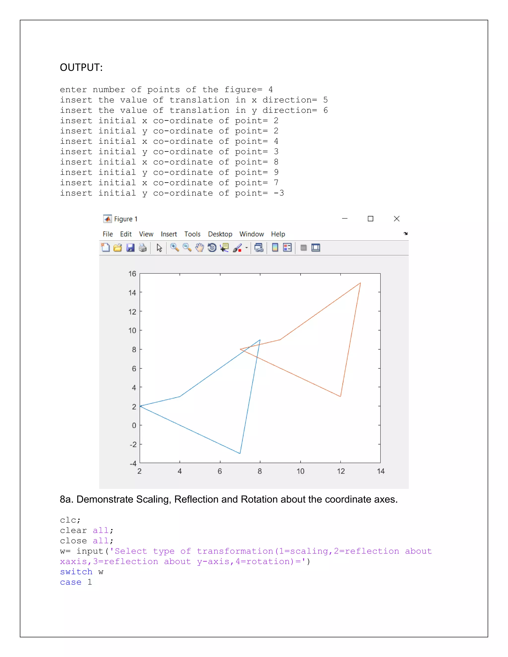
Exercise 8. Write a generalized code to perform a 2D translation on user specified
points (For line, triangle, and quadrilateral). Plot the figures before and after
transformation.
CODE:
clear all;
close all;
n= input('enter number of points of the figure= ');
tx= input('insert the value of translation in x direction= ');
ty= input('insert the value of translation in y direction= ');
for i=1:n
x(i)= input('insert initial x co-ordinate of point= ');
y(i)= input('insert initial y co-ordinate of point= ');
P(i,1)= [x(i)];
P(i,2)= [y(i)];
P(i,3)= [1];
end
P(n+1,1)=P(1,1);
P(n+1,2)=P(1,2);
P(n+1,3)= [1];
A= [1 0 0; 0 1 0;tx ty 1];
B= P*A;
B(n+1,1)=B(1,1);
B(n+1,2)=B(1,2);
B(n+1,3)= [1];
plot(P(:,1),P(:,2));
hold on;
plot(B(:,1),B(:,2));
8.
OUTPUT:
enter number ofpoints of the figure= 4
insert the value of translation in x direction= 5
insert the value of translation in y direction= 6
insert initial x co-ordinate of point= 2
insert initial y co-ordinate of point= 2
insert initial x co-ordinate of point= 4
insert initial y co-ordinate of point= 3
insert initial x co-ordinate of point= 8
insert initial y co-ordinate of point= 9
insert initial x co-ordinate of point= 7
insert initial y co-ordinate of point= -3
8a. Demonstrate Scaling, Reflection and Rotation about the coordinate axes.
clc;
clear all;
close all;
w= input('Select type of transformation(1=scaling,2=reflection about
xaxis,3=reflection about y-axis,4=rotation)=')
switch w
case 1
9.
n= input('enter numberof points of the figure= ');
ax= input('insert the value of scaling in x direction= ');
dy= input('insert the value of scaling in y direction= ');
for i=1:n
x(i)= input('insert initial x co-ordinate of point= ');
y(i)= input('insert initial y co-ordinate of point= ');
P(i,1)= [x(i)];
P(i,2)= [y(i)];
P(i,3)= [1];
end
P(n+1,1)=P(1,1);
P(n+1,2)=P(1,2);
P(n+1,3)= [1];
A= [ax 0 0; 0 dy 0;0 0 1];
B= P*A;
B(n+1,1)=B(1,1);
B(n+1,2)=B(1,2);
B(n+1,3)= [1];
plot(P(:,1),P(:,2));
hold on;
plot(B(:,1),B(:,2));
case 2
n= input('enter number of points of the figure= ');
for i=1:n
x(i)= input('insert initial x co-ordinate of point= ');
y(i)= input('insert initial y co-ordinate of point= ');
P(i,1)= [x(i)];
P(i,2)= [y(i)];
P(i,3)= [1];
end
P(n+1,1)=P(1,1);
P(n+1,2)=P(1,2);
P(n+1,3)= [1];
A= [1 0 0; 0 -1 0;0 0 1];
B= P*A;
B(n+1,1)=B(1,1);
B(n+1,2)=B(1,2);
B(n+1,3)= [1];
plot(P(:,1),P(:,2));
hold on;
plot(B(:,1),B(:,2));
case 3
n= input('enter number of points of the figure= ');
for i=1:n
x(i)= input('insert initial x co-ordinate of point= ');
y(i)= input('insert initial y co-ordinate of point= ');
P(i,1)= [x(i)];
P(i,2)= [y(i)];
P(i,3)= [1];
end
P(n+1,1)=P(1,1);
P(n+1,2)=P(1,2);
10.
P(n+1,3)= [1];
A= [-10 0; 0 1 0;0 0 1];
B= P*A;
B(n+1,1)=B(1,1);
B(n+1,2)=B(1,2);
B(n+1,3)= [1];
plot(P(:,1),P(:,2));
hold on;
plot(B(:,1),B(:,2));
case 4
n= input('enter number of points of the figure= ');
o= input('enter the angle of rotation= ')
for i=1:n
x(i)= input('insert initial x co-ordinate of point= ');
y(i)= input('insert initial y co-ordinate of point= ');
P(i,1)= [x(i)];
P(i,2)= [y(i)];
P(i,3)= [1];
end
P(n+1,1)=P(1,1);
P(n+1,2)=P(1,2);
P(n+1,3)= [1];
A= [1 0 0; 0 1 0;tx
ty 1];
B= P*A;
B(n+1,1)=B(1,1);
B(n+1,2)=B(1,2);
B(n+1,3)= [1];
plot(P(:,1),P(:,2));
hold on;
plot(B(:,1),B(:,2));
end
OUTPUT:
Select type of
transformation(1=scaling,2=reflection about xaxis,3=reflection about
y-axis,4=rotation)=1
enter number of points of the figure= 4
insert the value of scaling in x direction= 3
insert the value of scaling in y direction= 2
insert initial x co-ordinate of point= 2
insert initial y co-ordinate of point= 2
insert initial x co-ordinate of point= -3
insert initial y co-ordinate of point= 6
insert initial x co-ordinate of point= 5
insert initial y co-ordinate of point= 6
11.
insert initial xco-ordinate of point= 9
insert initial y co-ordinate of point= 11
Exercise 9: Write a generalized code to perform a 2D Rotation about an user specified
point on user specified entities (For line, triangle, and quadrilateral). Plot the figures
before and after transformation.
CODE:
clc;
clear all;
close all;
n=input('enter no of points on the figure ');
a=input('enter x coordinate o point about which entity is to be
rotated');
b=input('enter y coordinate o point about which entity is to be
rotated');
p=zeros(n,3);
for i=1:n
x(i)=input('enter x co-ordinate of point ');
y(i)=input('enter y co-ordinate of point ');
p(i,1)=[x(i)];
p(i,2)=[y(i)];
p(i,3)=[1];
end
p(n+1,1)=p(1,1);
p(n+1,2)=p(1,2);
d=input('angle to be rotated ');
rd=[cosd(d) sind(d) 0;-sind(d) cosd(d) 0;0 0 1];
t=[1 0 0;0 1 0;-a -b 1];
u=[1 0 0;0 1 0;a b 1];
q=p*t*rd*u
for j=1:n
r(j,1)=q(j,1);
r(j,2)=q(j,2);
end
r(n+1,1)=r(1,1);
r(n+1,2)=r(1,2);
plot(p(:,1),p(:,2))
hold on
plot(r(:,1),r(:,2))
OUTPUT:
enter no of points on the figure 3
enter x coordinate o point about which entity is to be rotated5
enter y coordinate o point about which entity is to be rotated5
enter x co-ordinate of point 1
12.
enter y co-ordinateof point 2
enter x co-ordinate of point 3
enter y co-ordinate of point 3
enter x co-ordinate of point 9
enter y co-ordinate of point 11
angle to be rotated 270
Exercise 10. Write a generalized code to demonstrate that the 3D Rotation is not
commutative. Use a simple rectangular parallelepiped to prove the same by plotting the
results.
function ret = rotate3(data,theta,axis)
%ROTATE3 Rotate points[data] in 3D about X, Y orZ axis by 'theta'
radians in CCW dir.
% Input: set of points, theta[angle of rotation] and axis
abbr.['x','y' or 'z'] about
% which the pionts are to be rotated
if nargin~=3
error('Enter set of points, angle of roation, and the axis to
ratate about');
end
13.
%creating matrix towork on
matrix = [data ones(size(data,1),1)];
%for easy use
ct = cos(theta);
st = sin(theta);
%deciding the matrix to use according to given parameter of axis
switch axis
case {'x','X'}
m_trans = [1 0 0 0; 0 ct -st 0; 0 st ct 0; 0 0 0 1];
case {'y', 'Y'}
m_trans = [ct 0 st 0; 0 1 0 0; -st 0 ct 0; 0 0 0 1];
case {'z', 'Z'}
m_trans = [ct -st 0 0; st ct 0 0; 0 0 1 0; 0 0 0 1];
otherwise
error('Choose axis from X Y or Z only!!')
end
%Calculating the multiplication and returning the data
ret = matrix*m_trans;
ret = ret(:,[1:3]);
end
Exercise 11: Design Problems
1. Develop a Matlab program with following details:
Design problem: Shaft
Input parameters: Power (KW), rpm of shaft, Allowable shear stress, factor of safety,
length of shaft
Output: diameter of shaft, weight of shaft.
CODE:
function FinalDimensions =
designShaft(power,rev_speed,tau,dia_ratio,length,rho)
%Calculating the torque first
power=power*1000;%kW to W
t = (60*power)/(2*pi*rev_speed);
t=t*1000;% Nm to Nmm
%From Strength criterion
FinalDimensions.OD = ((16*t)/(tau*pi*(1-dia_ratio^4)))^(1/3);%in mm
FinalDimensions.OD = ceil(FinalDimensions.OD); %rounding off
FinalDimensions.ID = floor(dia_ratio*FinalDimensions.OD);
FinalDimensions.wt = rho*pi*FinalDimensions.OD*FinalDimensions.OD*(1-
dia_ratio^2)*length;
FinalDimensions.wt = FinalDimensions.wt/10^9;%normalising to kg due to
OD taken in mm instead of m
14.
struct2table(FinalDimensions);
end
2. Develop aMatlab program by assuming same data as in problem 1 to find the
material saving if hollow shaft is used instead of solid shaft
CODE:
function [ output_args ] = Excercise11Question2( input_args )
%UNTITLED9 Summary of this function goes here
% Detailed explanation goes here
clc;
clear all;
P = input('Power (kW): ');
N = input('Speed (rpm): ');
Smax = input('Allowable Shear Stress (MPa): ');
FOS = input('Factor of safety: ');
L = input('Length of shaft (m):');
D = input('Density of the shaft material (kg/m^3): ');
k = input('Ratio of outer to inner diameter: ');
T = 60000*P/(2*pi*N);
d = ((16*T*FOS/(pi*Smax*1000000))^(1/3))*1000
d2 = ((16*k*T*FOS/(pi*Smax*(k^4-1)*1000000))^(1/3))*1000
d1 = k*d2
Weight_hollow = pi*((d1/1000)^2 - (d2/1000)^2)*L*D/4
Weight_Solid = pi*(d/1000)^2*L*D/4
Percentage_Material_Saving = (Weight_Solid-
Weight_hollow)*100/Weight_Solid
display '%';
end
3. Develop a Matlab program to design a cotter joint with following details:
Input: Material properties, load applied on cotter joint (tension and compression), factor
of safety for different parts
Output: All dimensions of cotter joint
CODE:
function FinalDimensions = designCotter(P)
%P is in kN
clc;
load matlab.mat
fprintf('nChoose a Material')
ff=MaterialProperties1(:,1);
%Make a selectable list assigning the values of Syt
Syt = 400; %N/mm^2
fosR = 6; %for spigot, socket and Rod
fosC = 4; %for Cotter
%permissible stresses for Rod
RsigmaT = Syt/fosR;
RsigmaC = 2*Syt/fosR;
15.
Rtau = Syt*0.5/fosR;
%permissiblestresses for Cotter
CsigmaT = Syt/fosC;
CsigmaC = 2*Syt/fosC;
Ctau = Syt*0.5/fosC;
CsigmaB = CsigmaT;
%Calculation of Dimensions
d = ceil(sqrt(4*P*1000/(pi*RsigmaT)))+1; %Dia of rods
t = ceil(0.31*d); %thk. of cotter
% P = [pi/4 d2^2 - d2*t]sigmaT
d2 = ceil(max(roots([pi/4,-t,-P*1000/RsigmaT])))+1; %Dia of Spigot
d1 = ceil(max(roots([pi/4,-t,(-P*1000/RsigmaT)+(-
pi*0.25*d2^2)+(t*d2)])))+3;%Dia of Socket outside
d3 = ceil(1.5*d); d4 = ceil(2.4*d)+3;%Spigot Collar d3 and Socket
Collar d4
a = ceil(.75*d); c = a;
b = ceil(max((P*1000/(2*Ctau*t)),sqrt((((d4-
d2)/6)+(d2/4))*3*P*1000/t/CsigmaB)));%Width of cotter (Shear vs
Bending)
%Cotter Length ??!!
l= 2*d4;
%Verification for crushing and shearing in spigot
flag=1;
if RsigmaC <= (P*1000/t/d2)
fprintf('nSpigot Failing under CRUSHING!')
flag = 0;
end
if Rtau <= (P*1000/2/a/d2)
fprintf('nSpigot Failing under SHEARING!')
flag = 0;
end
%Verification for crushing and shearing in socket
if RsigmaC <= (P*1000/t/(d4-d2))
fprintf('nSocket Failing under CRUSHING!')
flag = 0;
end
if Rtau <= (P*1000/2/c/(d4-d2))
fprintf('nSocket Failing under SHEARING!')
flag = 0;
end
%Spigot collar thk.
t1 = ceil(.45*d);
16.
if flag ==1
FinalDimensions.Parameter = {'Force Acting'; 'Diameter of Each
Rod'; 'Outside Diameter of Socket'; 'Diameter of Spigot or inside
diameter of Socket'; 'Diameter of Spigot-collar'; 'Diameter of Socket-
collar'; 'Distance from end of slot to the end of Spigot on Rod-B';
'Mean width of Cotter'; 'Axial distance from slot to end of Socket-
collar'; 'Thickness of Cotter'; 'Thickness of Spigot-collar'; 'Length
of Cotter'};
FinalDimensions.Value = [P; d; d1; d2; d3; d4; a; b; c; t; t1;
l];
FinalDimensions.Unit = {'(kN)'; '(mm)'; '(mm)'; '(mm)';
'(mm)'; '(mm)'; '(mm)'; '(mm)'; '(mm)'; '(mm)'; '(mm)'; '(mm)'};
FinalDimensions = struct2table(FinalDimensions);
end
fprintf('n')
4. Develop a Matlab code for the following data:
Objective: Selection of single row deep groove ball bearing
Input data: Radial load, axial load, expected life in hours, diameter of shaft
Output: Bearing designation
CODE:
clc;
clear all;
d=input('Enter the inner diameter of the shaft:');
Fr=input('Enter the radial load on bearing (kN):');
Fa=input('Enter the axial load on bearing (kN):');
Lh=input('Enter the expected life (hours):');
n=input('Enter the RPM:');
%the load factors assumed to be 1 each for both Fr and Fa
k=3;
P=Fr+Fa;
L=60*n*Lh;
co=(P*(L/(10^6))^(1/k));
switch d
case 25
if (co<4.36)
disp('The Bearing code is: 61805')
elseif (co>=4.36)&&(co<7.02)
disp('The Bearing code is: 61905')
elseif (co>=7.02)&&(co<8.06)
disp('The Bearing code is: 16005')
elseif (co>=8.06)&&(co<10.6)
disp('The Bearing code is: 68205')
elseif (co>=10.6)&&(co<11.9)
disp('The Bearing code is: 6005')
elseif (co>=11.9)&&(co<14.8)
disp('The Bearing code is: 6205')
elseif (co>=14.8)&&(co<17.8)
disp('The Bearing code is: 6205 ETN9')
17.
elseif (co>=17.8)&&(co<23.4)
disp('The Bearingcode is: 6305')
elseif (co>=23.4)&&(co<26)
disp('The Bearing code is: 6305 ETN9')
elseif (co>=26)&&(co<35.8)
disp('The Bearing code is: 6405')
else
disp('No bearings available for the given load and diameter')
end
case 28
if (co<16.8)
disp('The Bearing code is: 62/28')
elseif (co>=16.8)&&(co<25.1)
disp('The Bearing code is: 63/28')
else
disp('No Bearings available for the given load and
diameter.')
end
case 30
if (co<4.49)
disp('The Bearing code is: 61806')
elseif (co>=4.49)&&(co<7.28)
disp('The Bearing code is: 61906')
elseif (co>=7.28)&&(co<11.9)
disp('The Bearing code is: 16006')
elseif (co>=11.9)&&(co<13.8)
disp('The Bearing code is: 6006')
elseif (co>=13.8)&&(co<15.9)
disp('The Bearing code is: 98206')
elseif (co>=15.9)&&(co<20.3)
disp('The Bearing code is: 6206')
elseif (co>=20.3)&&(co<23.4)
disp('The Bearing code is: 6206 ETN9')
elseif (co>=23.4)&&(co<29.6)
disp('The Bearing code is: 6306 ')
elseif (co>=29.6)&&(co<32.5)
disp('The Bearing code is: 6306 ETN9')
elseif (co>=32.5)&&(co<43.6)
disp('The Bearing code is: 6406')
else
disp('There are no bearings available for the given load
carrying capacity and diameter.')
end
case 35
if (co<4.75)
disp('The Bearing code is: 61807')
elseif (co>=4.75)&&(co<9.56)
disp('The Bearing code is: 61907')
elseif (co>=9.56)&&(co<13)
disp('The Bearing code is: 16007')
elseif (co>=13)&&(co<16.8)
disp('The Bearing code is: 6007')
18.
elseif (co>=16.8)&&(co<27)
disp('The Bearingcode is: 6207')
elseif (co>=27)&&(co<31.2)
disp('The Bearing code is: 6207 ETN9')
elseif (co>=31.2)&&(co<35.1)
disp('The Bearing code is: 6307')
elseif (co>=35.1)&&(co<55.3)
disp('The Bearing code is: 6407')
else
disp('There are no bearings available for the given load
carrying capacity and diameter.')
end
otherwise
disp('Please enter a diameter from the above given options.')
end
![OUTPUT:
X1: 2
Y1: 6
X2: 9
Y2: 11
Exercise 7: Write a generalized code to generate a circle for a user specified radius and
coordinates of center point.
CODE:
clc;
clear all;
close all;
x1=input('x_centre: ');
y1=input('y_centre: ');
R=input('Radius: ');
x=0;
y=R;
p=1-R;
m=[x,y];
while(x<y)
x=x+1
if(p<0)
p=p+2*x+1
else
y=y-1
p=p+2*(x-y)+1
end
m=[m;x y]
end
m;
x=m(:,1);
y=m(:,2);
x2=x1+x;
y2=y1+y;
x3=x1-x;
y3=y1+y;](https://image.slidesharecdn.com/matlabassignment-210517073943/75/Matlab-assignment-4-2048.jpg)
![m = 0 8
1 8
2 8
3 7
4 7
5 6
6 5
Exercise 8. Write a generalized code to perform a 2D translation on user specified
points (For line, triangle, and quadrilateral). Plot the figures before and after
transformation.
CODE:
clear all;
close all;
n= input('enter number of points of the figure= ');
tx= input('insert the value of translation in x direction= ');
ty= input('insert the value of translation in y direction= ');
for i=1:n
x(i)= input('insert initial x co-ordinate of point= ');
y(i)= input('insert initial y co-ordinate of point= ');
P(i,1)= [x(i)];
P(i,2)= [y(i)];
P(i,3)= [1];
end
P(n+1,1)=P(1,1);
P(n+1,2)=P(1,2);
P(n+1,3)= [1];
A= [1 0 0; 0 1 0;tx ty 1];
B= P*A;
B(n+1,1)=B(1,1);
B(n+1,2)=B(1,2);
B(n+1,3)= [1];
plot(P(:,1),P(:,2));
hold on;
plot(B(:,1),B(:,2));](https://image.slidesharecdn.com/matlabassignment-210517073943/75/Matlab-assignment-7-2048.jpg)
![n= input('enter number of points of the figure= ');
ax= input('insert the value of scaling in x direction= ');
dy= input('insert the value of scaling in y direction= ');
for i=1:n
x(i)= input('insert initial x co-ordinate of point= ');
y(i)= input('insert initial y co-ordinate of point= ');
P(i,1)= [x(i)];
P(i,2)= [y(i)];
P(i,3)= [1];
end
P(n+1,1)=P(1,1);
P(n+1,2)=P(1,2);
P(n+1,3)= [1];
A= [ax 0 0; 0 dy 0;0 0 1];
B= P*A;
B(n+1,1)=B(1,1);
B(n+1,2)=B(1,2);
B(n+1,3)= [1];
plot(P(:,1),P(:,2));
hold on;
plot(B(:,1),B(:,2));
case 2
n= input('enter number of points of the figure= ');
for i=1:n
x(i)= input('insert initial x co-ordinate of point= ');
y(i)= input('insert initial y co-ordinate of point= ');
P(i,1)= [x(i)];
P(i,2)= [y(i)];
P(i,3)= [1];
end
P(n+1,1)=P(1,1);
P(n+1,2)=P(1,2);
P(n+1,3)= [1];
A= [1 0 0; 0 -1 0;0 0 1];
B= P*A;
B(n+1,1)=B(1,1);
B(n+1,2)=B(1,2);
B(n+1,3)= [1];
plot(P(:,1),P(:,2));
hold on;
plot(B(:,1),B(:,2));
case 3
n= input('enter number of points of the figure= ');
for i=1:n
x(i)= input('insert initial x co-ordinate of point= ');
y(i)= input('insert initial y co-ordinate of point= ');
P(i,1)= [x(i)];
P(i,2)= [y(i)];
P(i,3)= [1];
end
P(n+1,1)=P(1,1);
P(n+1,2)=P(1,2);](https://image.slidesharecdn.com/matlabassignment-210517073943/75/Matlab-assignment-9-2048.jpg)
![P(n+1,3)= [1];
A= [-1 0 0; 0 1 0;0 0 1];
B= P*A;
B(n+1,1)=B(1,1);
B(n+1,2)=B(1,2);
B(n+1,3)= [1];
plot(P(:,1),P(:,2));
hold on;
plot(B(:,1),B(:,2));
case 4
n= input('enter number of points of the figure= ');
o= input('enter the angle of rotation= ')
for i=1:n
x(i)= input('insert initial x co-ordinate of point= ');
y(i)= input('insert initial y co-ordinate of point= ');
P(i,1)= [x(i)];
P(i,2)= [y(i)];
P(i,3)= [1];
end
P(n+1,1)=P(1,1);
P(n+1,2)=P(1,2);
P(n+1,3)= [1];
A= [1 0 0; 0 1 0;tx
ty 1];
B= P*A;
B(n+1,1)=B(1,1);
B(n+1,2)=B(1,2);
B(n+1,3)= [1];
plot(P(:,1),P(:,2));
hold on;
plot(B(:,1),B(:,2));
end
OUTPUT:
Select type of
transformation(1=scaling,2=reflection about xaxis,3=reflection about
y-axis,4=rotation)=1
enter number of points of the figure= 4
insert the value of scaling in x direction= 3
insert the value of scaling in y direction= 2
insert initial x co-ordinate of point= 2
insert initial y co-ordinate of point= 2
insert initial x co-ordinate of point= -3
insert initial y co-ordinate of point= 6
insert initial x co-ordinate of point= 5
insert initial y co-ordinate of point= 6](https://image.slidesharecdn.com/matlabassignment-210517073943/75/Matlab-assignment-10-2048.jpg)
![insert initial x co-ordinate of point= 9
insert initial y co-ordinate of point= 11
Exercise 9: Write a generalized code to perform a 2D Rotation about an user specified
point on user specified entities (For line, triangle, and quadrilateral). Plot the figures
before and after transformation.
CODE:
clc;
clear all;
close all;
n=input('enter no of points on the figure ');
a=input('enter x coordinate o point about which entity is to be
rotated');
b=input('enter y coordinate o point about which entity is to be
rotated');
p=zeros(n,3);
for i=1:n
x(i)=input('enter x co-ordinate of point ');
y(i)=input('enter y co-ordinate of point ');
p(i,1)=[x(i)];
p(i,2)=[y(i)];
p(i,3)=[1];
end
p(n+1,1)=p(1,1);
p(n+1,2)=p(1,2);
d=input('angle to be rotated ');
rd=[cosd(d) sind(d) 0;-sind(d) cosd(d) 0;0 0 1];
t=[1 0 0;0 1 0;-a -b 1];
u=[1 0 0;0 1 0;a b 1];
q=p*t*rd*u
for j=1:n
r(j,1)=q(j,1);
r(j,2)=q(j,2);
end
r(n+1,1)=r(1,1);
r(n+1,2)=r(1,2);
plot(p(:,1),p(:,2))
hold on
plot(r(:,1),r(:,2))
OUTPUT:
enter no of points on the figure 3
enter x coordinate o point about which entity is to be rotated5
enter y coordinate o point about which entity is to be rotated5
enter x co-ordinate of point 1](https://image.slidesharecdn.com/matlabassignment-210517073943/75/Matlab-assignment-11-2048.jpg)
![enter y co-ordinate of point 2
enter x co-ordinate of point 3
enter y co-ordinate of point 3
enter x co-ordinate of point 9
enter y co-ordinate of point 11
angle to be rotated 270
Exercise 10. Write a generalized code to demonstrate that the 3D Rotation is not
commutative. Use a simple rectangular parallelepiped to prove the same by plotting the
results.
function ret = rotate3(data,theta,axis)
%ROTATE3 Rotate points[data] in 3D about X, Y orZ axis by 'theta'
radians in CCW dir.
% Input: set of points, theta[angle of rotation] and axis
abbr.['x','y' or 'z'] about
% which the pionts are to be rotated
if nargin~=3
error('Enter set of points, angle of roation, and the axis to
ratate about');
end](https://image.slidesharecdn.com/matlabassignment-210517073943/75/Matlab-assignment-12-2048.jpg)
![%creating matrix to work on
matrix = [data ones(size(data,1),1)];
%for easy use
ct = cos(theta);
st = sin(theta);
%deciding the matrix to use according to given parameter of axis
switch axis
case {'x','X'}
m_trans = [1 0 0 0; 0 ct -st 0; 0 st ct 0; 0 0 0 1];
case {'y', 'Y'}
m_trans = [ct 0 st 0; 0 1 0 0; -st 0 ct 0; 0 0 0 1];
case {'z', 'Z'}
m_trans = [ct -st 0 0; st ct 0 0; 0 0 1 0; 0 0 0 1];
otherwise
error('Choose axis from X Y or Z only!!')
end
%Calculating the multiplication and returning the data
ret = matrix*m_trans;
ret = ret(:,[1:3]);
end
Exercise 11: Design Problems
1. Develop a Matlab program with following details:
Design problem: Shaft
Input parameters: Power (KW), rpm of shaft, Allowable shear stress, factor of safety,
length of shaft
Output: diameter of shaft, weight of shaft.
CODE:
function FinalDimensions =
designShaft(power,rev_speed,tau,dia_ratio,length,rho)
%Calculating the torque first
power=power*1000;%kW to W
t = (60*power)/(2*pi*rev_speed);
t=t*1000;% Nm to Nmm
%From Strength criterion
FinalDimensions.OD = ((16*t)/(tau*pi*(1-dia_ratio^4)))^(1/3);%in mm
FinalDimensions.OD = ceil(FinalDimensions.OD); %rounding off
FinalDimensions.ID = floor(dia_ratio*FinalDimensions.OD);
FinalDimensions.wt = rho*pi*FinalDimensions.OD*FinalDimensions.OD*(1-
dia_ratio^2)*length;
FinalDimensions.wt = FinalDimensions.wt/10^9;%normalising to kg due to
OD taken in mm instead of m](https://image.slidesharecdn.com/matlabassignment-210517073943/75/Matlab-assignment-13-2048.jpg)
![struct2table(FinalDimensions);
end
2. Develop a Matlab program by assuming same data as in problem 1 to find the
material saving if hollow shaft is used instead of solid shaft
CODE:
function [ output_args ] = Excercise11Question2( input_args )
%UNTITLED9 Summary of this function goes here
% Detailed explanation goes here
clc;
clear all;
P = input('Power (kW): ');
N = input('Speed (rpm): ');
Smax = input('Allowable Shear Stress (MPa): ');
FOS = input('Factor of safety: ');
L = input('Length of shaft (m):');
D = input('Density of the shaft material (kg/m^3): ');
k = input('Ratio of outer to inner diameter: ');
T = 60000*P/(2*pi*N);
d = ((16*T*FOS/(pi*Smax*1000000))^(1/3))*1000
d2 = ((16*k*T*FOS/(pi*Smax*(k^4-1)*1000000))^(1/3))*1000
d1 = k*d2
Weight_hollow = pi*((d1/1000)^2 - (d2/1000)^2)*L*D/4
Weight_Solid = pi*(d/1000)^2*L*D/4
Percentage_Material_Saving = (Weight_Solid-
Weight_hollow)*100/Weight_Solid
display '%';
end
3. Develop a Matlab program to design a cotter joint with following details:
Input: Material properties, load applied on cotter joint (tension and compression), factor
of safety for different parts
Output: All dimensions of cotter joint
CODE:
function FinalDimensions = designCotter(P)
%P is in kN
clc;
load matlab.mat
fprintf('nChoose a Material')
ff=MaterialProperties1(:,1);
%Make a selectable list assigning the values of Syt
Syt = 400; %N/mm^2
fosR = 6; %for spigot, socket and Rod
fosC = 4; %for Cotter
%permissible stresses for Rod
RsigmaT = Syt/fosR;
RsigmaC = 2*Syt/fosR;](https://image.slidesharecdn.com/matlabassignment-210517073943/75/Matlab-assignment-14-2048.jpg)
![Rtau = Syt*0.5/fosR;
%permissible stresses for Cotter
CsigmaT = Syt/fosC;
CsigmaC = 2*Syt/fosC;
Ctau = Syt*0.5/fosC;
CsigmaB = CsigmaT;
%Calculation of Dimensions
d = ceil(sqrt(4*P*1000/(pi*RsigmaT)))+1; %Dia of rods
t = ceil(0.31*d); %thk. of cotter
% P = [pi/4 d2^2 - d2*t]sigmaT
d2 = ceil(max(roots([pi/4,-t,-P*1000/RsigmaT])))+1; %Dia of Spigot
d1 = ceil(max(roots([pi/4,-t,(-P*1000/RsigmaT)+(-
pi*0.25*d2^2)+(t*d2)])))+3;%Dia of Socket outside
d3 = ceil(1.5*d); d4 = ceil(2.4*d)+3;%Spigot Collar d3 and Socket
Collar d4
a = ceil(.75*d); c = a;
b = ceil(max((P*1000/(2*Ctau*t)),sqrt((((d4-
d2)/6)+(d2/4))*3*P*1000/t/CsigmaB)));%Width of cotter (Shear vs
Bending)
%Cotter Length ??!!
l= 2*d4;
%Verification for crushing and shearing in spigot
flag=1;
if RsigmaC <= (P*1000/t/d2)
fprintf('nSpigot Failing under CRUSHING!')
flag = 0;
end
if Rtau <= (P*1000/2/a/d2)
fprintf('nSpigot Failing under SHEARING!')
flag = 0;
end
%Verification for crushing and shearing in socket
if RsigmaC <= (P*1000/t/(d4-d2))
fprintf('nSocket Failing under CRUSHING!')
flag = 0;
end
if Rtau <= (P*1000/2/c/(d4-d2))
fprintf('nSocket Failing under SHEARING!')
flag = 0;
end
%Spigot collar thk.
t1 = ceil(.45*d);](https://image.slidesharecdn.com/matlabassignment-210517073943/75/Matlab-assignment-15-2048.jpg)
![if flag == 1
FinalDimensions.Parameter = {'Force Acting'; 'Diameter of Each
Rod'; 'Outside Diameter of Socket'; 'Diameter of Spigot or inside
diameter of Socket'; 'Diameter of Spigot-collar'; 'Diameter of Socket-
collar'; 'Distance from end of slot to the end of Spigot on Rod-B';
'Mean width of Cotter'; 'Axial distance from slot to end of Socket-
collar'; 'Thickness of Cotter'; 'Thickness of Spigot-collar'; 'Length
of Cotter'};
FinalDimensions.Value = [P; d; d1; d2; d3; d4; a; b; c; t; t1;
l];
FinalDimensions.Unit = {'(kN)'; '(mm)'; '(mm)'; '(mm)';
'(mm)'; '(mm)'; '(mm)'; '(mm)'; '(mm)'; '(mm)'; '(mm)'; '(mm)'};
FinalDimensions = struct2table(FinalDimensions);
end
fprintf('n')
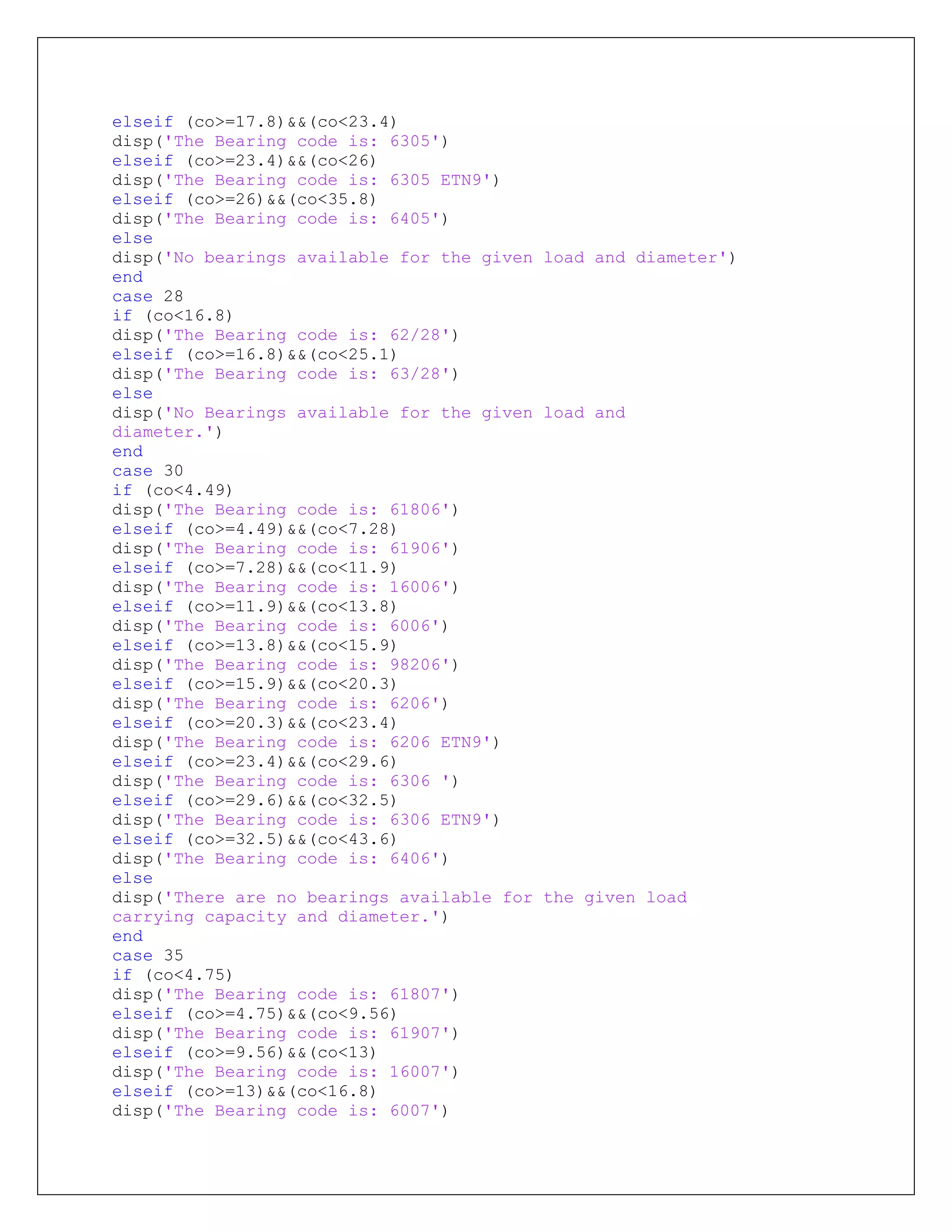
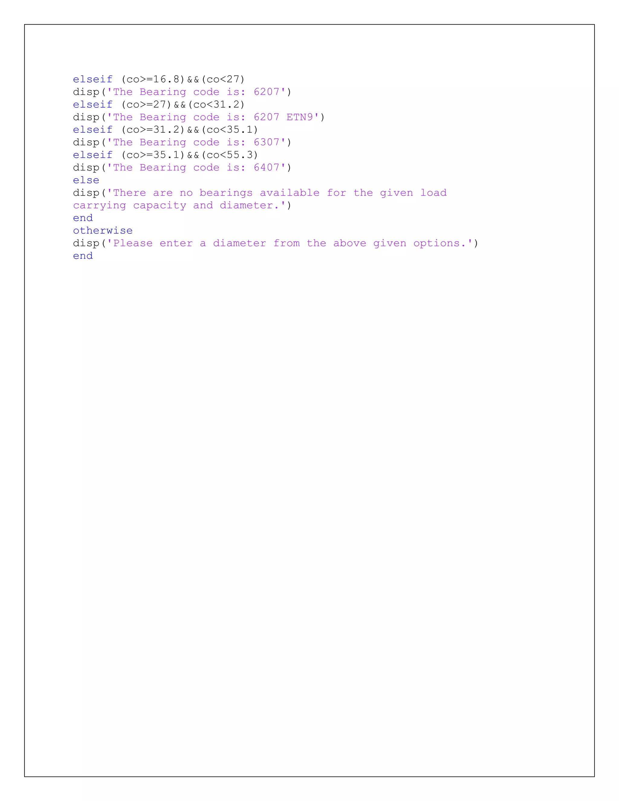
4. Develop a Matlab code for the following data:
Objective: Selection of single row deep groove ball bearing
Input data: Radial load, axial load, expected life in hours, diameter of shaft
Output: Bearing designation
CODE:
clc;
clear all;
d=input('Enter the inner diameter of the shaft:');
Fr=input('Enter the radial load on bearing (kN):');
Fa=input('Enter the axial load on bearing (kN):');
Lh=input('Enter the expected life (hours):');
n=input('Enter the RPM:');
%the load factors assumed to be 1 each for both Fr and Fa
k=3;
P=Fr+Fa;
L=60*n*Lh;
co=(P*(L/(10^6))^(1/k));
switch d
case 25
if (co<4.36)
disp('The Bearing code is: 61805')
elseif (co>=4.36)&&(co<7.02)
disp('The Bearing code is: 61905')
elseif (co>=7.02)&&(co<8.06)
disp('The Bearing code is: 16005')
elseif (co>=8.06)&&(co<10.6)
disp('The Bearing code is: 68205')
elseif (co>=10.6)&&(co<11.9)
disp('The Bearing code is: 6005')
elseif (co>=11.9)&&(co<14.8)
disp('The Bearing code is: 6205')
elseif (co>=14.8)&&(co<17.8)
disp('The Bearing code is: 6205 ETN9')](https://image.slidesharecdn.com/matlabassignment-210517073943/75/Matlab-assignment-16-2048.jpg)