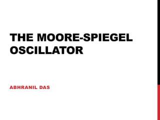
![Roots for T=6 and R=20
Root Seed (Newton- Interval
Raphson) (Bisection)
3 5 [0,5]
0.4495 0 [0,1]
-4.4495 -5 [-5,0]](https://image.slidesharecdn.com/themoore-spiegeloscillator-120901062409-phpapp01/85/The-Moore-Spiegel-Oscillator-5-320.jpg)
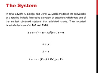
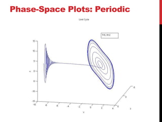
![Phase-Space Plots with RK4/5 (General Code)
t=10; N=10000; h=float(t)/N; l=range(3)
T=6; R=20
x=list(input('Starting x,y,z: '))
file=open('msplot.txt', 'w')
def f(x):
return [x[1], x[2], -x[2]-(T-R+R*x[0]**2)*x[1]-T*x[0]]
for iter in range(N):
print>> file, x[0],x[1],x[2]
k1=[h*f(x)[i] for i in l]
k2=[h*f([(x[j]+k1[j]/2) for j in l])[i] for i in l]
k3=[h*f([(x[j]+k2[j]/2) for j in l])[i] for i in l]
k4=[h*f([(x[j]+k3[j]) for j in l])[i] for i in l]
x=[x[i]+(k1[i]+2*k2[i]+2*k3[i]+k4[i]) for i in l]
file.close()
import Gnuplot
g=Gnuplot.Gnuplot()
g('''splot 'msplot.txt' w l''')
g('pause -1')
global T;
global R;
T=0;
R=20;
[tarray,Y] = ode45(@mseq,[0 1000],[-1 1 0]);
function dy = mseq(t,y)
global T;
global R;
dy = zeros(3,1);
dy(1) = y(2);
dy(2) = y(3);
dy(3) = -y(3)-(T-R+R*y(1)^2)*y(2)-T*y(1);
end](https://image.slidesharecdn.com/themoore-spiegeloscillator-120901062409-phpapp01/85/The-Moore-Spiegel-Oscillator-6-320.jpg)
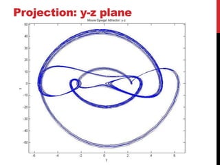
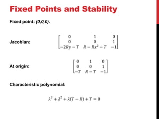
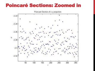
![Poincaré Sections of projections
P=[];
for i=1:length(Y)-1
if (Y(i,2))<0 && (Y(i+1,2))>0
P(end+1)=Y(i,1);
end
end
P=P';
plot(P,'.');](https://image.slidesharecdn.com/themoore-spiegeloscillator-120901062409-phpapp01/85/The-Moore-Spiegel-Oscillator-15-320.jpg)
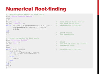
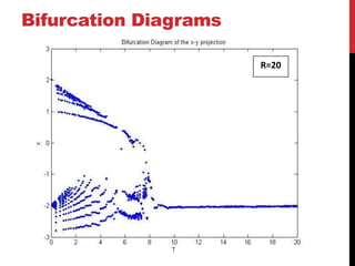
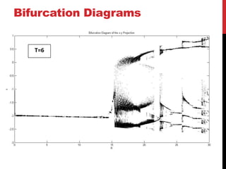
![Bifurcation Diagrams
global T;
global R;
T=0;
R=20;
B=[];
while T<20
[tarray,Y] = ode45(@mseq,[0 1000],[-1 1 0]);
P=[];
for i=1:length(Y)-1
if (Y(i,2))<0 && (Y(i+1,2))>0
P(end+1)=Y(i,1);
end
end
P=P';
P=P(end-10:end);
for i=1:length(P)
B(end+1,:)=[T P(i)];
end
T=T+.1
end](https://image.slidesharecdn.com/themoore-spiegeloscillator-120901062409-phpapp01/85/The-Moore-Spiegel-Oscillator-17-320.jpg)

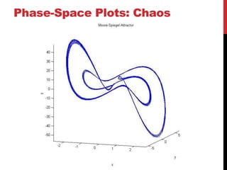
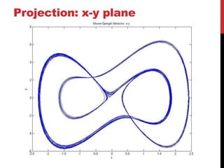
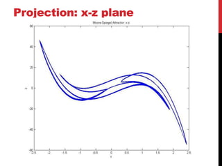
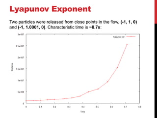
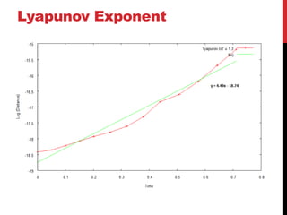
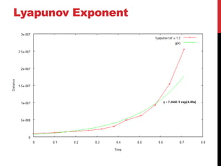
This document discusses the Moore-Spiegel oscillator, a nonlinear oscillator model used to study chaos. It provides the system equations, finds periodic and chaotic solutions using numerical integration, and analyzes the dynamics through phase space plots, Poincare sections, bifurcation diagrams, and Lyapunov exponents. The analysis reveals transitions from periodic to chaotic behavior as the control parameters are varied.


