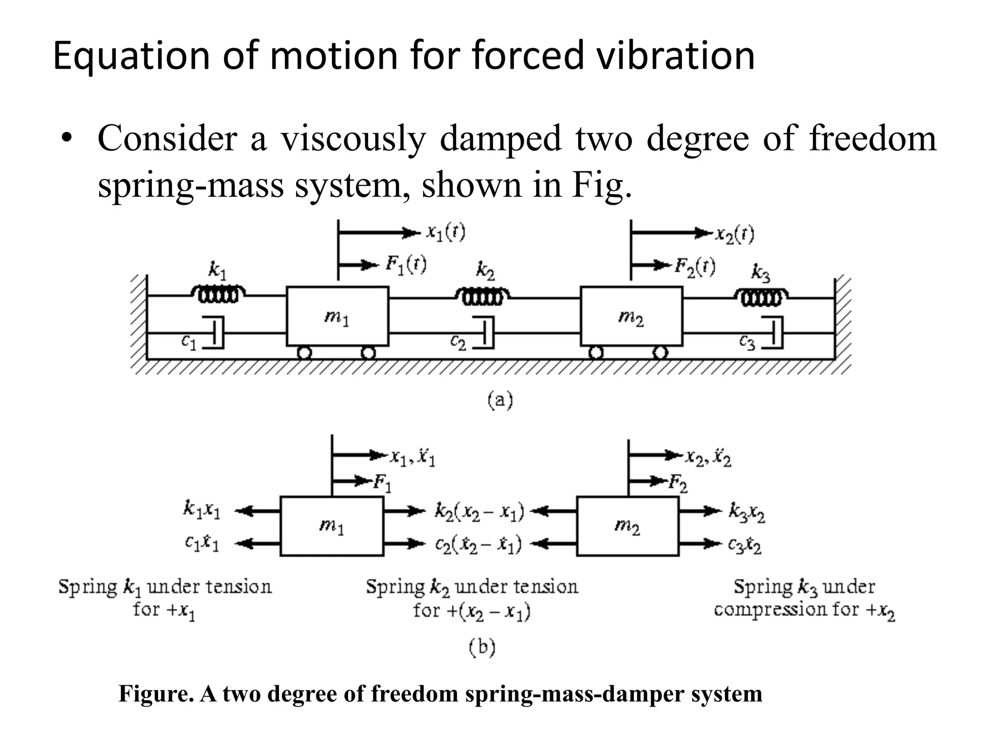
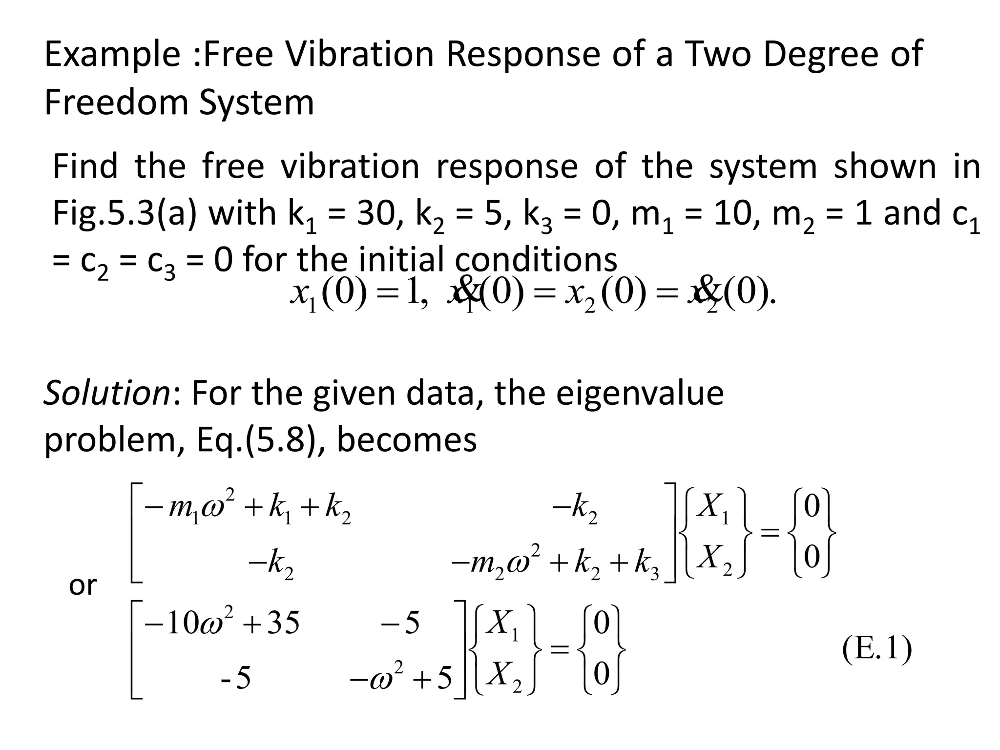
GANDHINAGAR INSTITUTE
OF TECHNOLOGY
Subject: Dynamics of machine
Topic:-Two degree of freedom system
Branch:-Mechanical
Sem.:-6
Div:-D
Prepared By:- Guided By:-
Patel Yash S. (150123119039) Prof. Samir Raval
INTRODUCTION
• The System which require two independent
co-ordinates to specify its motion at
configuration at instant is called two degree of
freedom system.
– Example: motor pump system.
• There are two equations of motion for a 2DOF
system, one for each mass (more precisely, for
each DOF).
• They are generally in the form of couple
differential equation that is, each equation
involves all the coordinates.
Equation of motion for forced vibration
• Consider a viscously damped two degree of freedom
spring-mass system, shown in Fig.
Figure. A two degree of freedom spring-mass-damper system
Equations of Motion for Forced Vibration
)2.5()()(
)1.5()()(
2232122321222
1221212212111
Fxkkxkxccxcxm
Fxkxkkxcxccxm




)3.5()()(][)(][)(][ tFtxktxctxm


Both equations can be written in matrix form as
The application of Newton’s second law of motion to each
of the masses gives the equations of motion:
where [m], [c], and [k] are called the mass, damping,
and stiffness matrices, respectively, and are given by
Equations of Motion for Forced Vibration
























322
221
322
221
2
1
][
][
0
0
][
kkk
kkk
k
ccc
ccc
c
m
m
m














)(
)(
)(
)(
)(
)(
2
1
2
1
tF
tF
tF
tx
tx
tx

And the displacement and force vectors are given
respectively:
It can be seen that the matrices [m], [c], and [k] are all 2 x
2 matrices whose elements are known masses, damping
coefficient and stiffnesses of the system, respectively.
Equations of Motion for Forced Vibration
][][],[][],[][ kkccmm TTT

6
where the superscript T denotes the transpose of the
matrix.
oThe solution of Eqs.(5.1) and (5.2) involves four
constants of integration (two for each equation). Usually
the initial displacements and velocities of the two masses
are specified as
oFurther, these matrices can be seen to be symmetric,
so that,
x1(t = 0) = x1(0) and 1( t = 0) = 1(0),
x2(t = 0) = x2(0) and 2 (t = 0) = 2(0).
x
x x
x
Free Vibration Analysis of an Undamped System
)5.5(0)()()()(
)4.5(0)()()()(
2321222
2212111


txkktxktxm
txktxkktxm


)6.5()cos()(
)cos()(
22
11




tXtx
tXtx
7
Assuming that it is possible to have harmonic motion of
m1 and m2 at the same frequency ω and the same phase
angle Φ, we take the solutions as
By setting F1(t) = F2(t) = 0, and damping disregarded, i.e.,
c1 = c2 = c3 = 0, and the equation of motion is reduced to:
Free Vibration Analysis of an Undamped System
  
   )7.5(0)cos()(
0)cos()(
232
2
212
22121
2
1




tXkkmXk
tXkXkkm
 
  )8.5(0)(
0)(
232
2
212
22121
2
1


XkkmXk
XkXkkm


Since Eq.(5.7)must be satisfied for all values of the time t,
the terms between brackets must be zero. Thus,
Substituting into Eqs.(5.4) and (5.5),
Free Vibration Analysis of an Undamped System
 
 
0
)(
)(
det
21
2
12
221
2
1











kkmk
kkkm


 
  )9.5(0))((
)()()(
2
23221
132221
4
21


kkkkk
mkkmkkmm 
or
which represent two simultaneous homogenous algebraic
equations in the unknown X1 and X2. For trivial solution,
i.e., X1 = X2 = 0, there is no solution. For a nontrivial
solution, the determinant of the coefficients of X1 and X2
must be zero:
)10.5(
))((
4
)()(
2
1
)()(
2
1
,
2/1
21
2
23221
2
21
132221
21
1322212
2
2
1





 










 





 

mm
kkkkk
mm
mkkmkk
mm
mkkmkk


The roots are called natural frequencies of the system.
which is called the frequency or characteristic equation.
Hence the roots are:
FREE VIBRATION ANALYSIS OF AN UNDAMPED SYSTEM
Free Vibration Analysis of an Undamped System
)11.5(
)(
)(
)(
)(
32
2
22
2
2
21
2
21
)2(
1
)2(
2
2
32
2
12
2
2
21
2
11
)1(
1
)1(
2
1
kkm
k
k
kkm
X
X
r
kkm
k
k
kkm
X
X
r












)12.5(and )2(
12
)2(
1
)2(
2
)2(
1)2(
)1(
11
)1(
1
)1(
2
)1(
1)1(




































Xr
X
X
X
X
Xr
X
X
X
X

The normal modes of vibration corresponding to ω1
2
and ω2
2 can be expressed, respectively, as
To determine the values of X1 and X2, given ratio
which are known as the modal vectors of the system.
Free Vibration Analysis of an Undamped System
(5.17)modesecond
)cos(
)cos(
)(
)(
)(
modefirst
)cos(
)cos(
)(
)(
)(
22
)2(
12
22
)2(
1
)2(
2
)2(
1)2(
11
)1(
11
11
)1(
1
)1(
2
)1(
1)1(














































tXr
tX
tx
tx
tx
tXr
tX
tx
tx
tx


0)0(,)0(
,0)0(constant,some)0(
2
)(
12
1
)(
11


txXrtx
txXtx
i
i
i


Where the constants , , and are determined by
the initial conditions. The initial conditions are
The free vibration solution or the motion in time can be
expressed itself as
)1(
1X )2(
1X 1 2
Free Vibration Analysis of an Undamped System
)14.5()()()( 2211 txctxctx


)15.5()cos()cos(
)()()(
)cos()cos()()()(
22
)2(
1211
)1(
11
)2(
2
)1(
22
22
)2(
111
)1(
1
)2(
1
)1(
11





tXrtXr
txtxtx
tXtXtxtxtx
Thus the components of the vector can be expressed as
The resulting motion can be obtained by a linear
superposition of the two normal modes, Eq.(5.13)
where the unknown constants can be determined from
the initial conditions:
Free Vibration Analysis of an Undamped System
)16.5()0()0(),0()0(
),0()0(),0()0(
2222
1111
xtxxtx
xtxxtx




)17.5(sinsin)0(
coscos)0(
sinsin)0(
coscos)0(
2
)2(
1221
)1(
1112
2
)2(
121
)1(
112
2
)2(
121
)1(
111
2
)2(
11
)1(
11




XrXrx
XrXrx
XXx
XXx










































)(
)0()0(
sin,
)(
)0()0(
sin
)0()0(
cos,
)0()0(
cos
122
211
2
)2(
1
121
212
1
)1(
1
12
211
2
)2(
1
12
212
1
)1(
1
rr
xxr
X
rr
xxr
X
rr
xxr
X
rr
xxr
X






Substituting into Eq.(5.15) leads to
The solution can be expressed as
Free Vibration Analysis of an Undamped System
    
   
    
   
)18.5(
)0()0([
)0()0(
tan
cos
sin
tan
)0()0([
)0()0(
tan
cos
sin
tan
)0()0(
)0()0(
)(
1
sincos
)0()0(
)0()0(
)(
1
sincos
2112
2111
2
)2(
1
2
)2(
11
2
2121
2121
1
)1(
1
1
)1(
11
1
2/1
2
2
2
2112
211
12
2/12
2
)2(
1
2
2
)2(
1
)2(
1
2/1
2
1
2
2122
212
12
2/12
1
)1(
1
2
1
)1(
1
)1(
1





































 









 






xxr
xxr
X
X
xxr
xxr
X
X
xxr
xxr
rr
XXX
xxr
xxr
rr
XXX














from which we obtain the desired solution
Example :Free Vibration Response of a Two Degree of
Freedom System
).0()0()0(,1)0( 2211 xxxx  
(E.1)
0
0
55-
53510
0
0
2
1
2
2
2
1
32
2
22
221
2
1














































X
X
X
X
kkmk
kkkm




Solution: For the given data, the eigenvalue
problem, Eq.(5.8), becomes
Find the free vibration response of the system shown in
Fig.5.3(a) with k1 = 30, k2 = 5, k3 = 0, m1 = 10, m2 = 1 and c1
= c2 = c3 = 0 for the initial conditions
or
Solution
(E.2)01508510 24
 
E.3)(4495.2,5811.1
0.6,5.2
21
2
2
2
1




E.5)(
5
1
E.4)(
2
1
)2(
1)2(
2
)2(
1)2(
)1(
1)1(
2
)1(
1)1(
X
X
X
X
X
X
X
X



































from which the natural frequencies can be found as
By setting the determinant of the coefficient matrix in
Eq.(E.1) to zero, we obtain the frequency equation,
The normal modes (or eigenvectors) are given by
Solution
(E.7))4495.2cos(5)5811.1cos(2)(
(E.6))4495.2cos()5811.1cos()(
2
)2(
11
)1(
12
2
)2(
11
)1(
11




tXtXtx
tXtXtx
(E.11)sin2475.121622.3)0(
(E.10)sin4495.2sin5811.10)0(
(E.9)cos5cos20)0(
(E.8)coscos1)0(
2
)2(
1
)1(
12
2
)2(
11
)1(
11
2
)2(
11
)1(
12
2
)2(
11
)1(
11




XXtx
XXtx
XXtx
XXtx






By using the given initial conditions in Eqs.(E.6) and
(E.7), we obtain
The free vibration responses of the masses m1 and m2
are given by (see Eq.5.15):
Solution
(E.12)
7
2
cos;
7
5
cos 2
)2(
11
)1(
1   XX
(E.13)0sin,0sin 2
)2(
11
)1(
1   XX
(E.14)0,0,
7
2
,
7
5
21
)2(
1
)1(
1  XX
while the solution of Eqs.(E.10) and (E.11) leads to
The solution of Eqs.(E.8) and (E.9) yields
Equations (E.12) and (E.13) give
Solution
(E.16)4495.2cos
7
10
5811.1cos
7
10
)(
(E.15)4495.2cos
7
2
5811.1cos
7
5
)(
2
1
tttx
tttx


Thus the free vibration responses of m1 and m2 are
given by
Torsional System
Figure : Torsional system with discs mounted on a shaft
Consider a torsional system as shown in Fig. The
differential equations of rotational motion for the discs
can be derived as
Torsional System
22312222
11221111
)(
)(
ttt
ttt
MkkJ
MkkJ






)19.5()(
)(
22321222
12212111
tttt
tttt
MkkkJ
MkkkJ






which upon rearrangement become
For the free vibration analysis of the system, Eq.(5.19)
reduces to
)20.5(0)(
0)(
2321222
2212111




ttt
ttt
kkkJ
kkkJ


Coordinate Coupling and Principal Coordinates
Generalized coordinates are sets of n coordinates used
to describe the configuration of the system.
•Equations of motion Using x(t) and θ(t).
Coordinate Coupling and Principal Coordinates
)21.5()()( 2211  lxklxkxm 
)22.5()()( 2221110 llxkllxkJ  
and the moment equation about C.G. can be expressed
as
From the free-body diagram shown in Fig.5.10a, with
the positive values of the motion variables as indicated,
the force equilibrium equation in the vertical direction
can be written as
Eqs.(5.21) and (5.22) can be rearranged and written in
matrix form as
Coordinate Coupling and Principal Coordinates
)23.5(
0
0
)()(
)()(
0
0
2
2
2
12211
221121
0 21 




































x
lklklklk
lklkkkx
J
m


  melyklykym  )()( 2211
The lathe rotates in the vertical plane and has vertical
motion as well, unless k1l1 = k2l2. This is known as
elastic or static coupling.
From Fig.5.10b, the equations of motion for translation
and rotation can be written as
•Equations of motion Using y(t) and θ(t).
Coordinate Coupling and Principal Coordinates
)24.5()()( 222111 ymellykllykJP
  
)25.5(
0
0
)()(
)()(
2
2
2
112211
112221
2 




































y
lklklklk
lklkkky
Jme
mem
P


2211 lklk 
These equations can be rearranged and written in
matrix form as
If , the system will have dynamic or inertia
coupling only.
Note the following characteristics of these systems:
Coordinate Coupling and Principal Coordinates
)26.5(
0
0
2
1
2221
1211
2
1
2221
1211
2
1
2221
1211













































x
x
kk
kk
x
x
cc
cc
x
x
mm
mm




1. In the most general case, a viscously damped two
degree of freedom system has the equations of
motions in the form:
2. The system vibrates in its own natural way regardless
of the coordinates used. The choice of the coordinates
is a mere convenience.
3. Principal or natural coordinates are defined as system
of coordinates which give equations of motion that are
uncoupled both statically and dynamically.
Example :Principal Coordinates of Spring-Mass System
Determine the principal coordinates for the spring-mass
system shown in Fig.
Solution
(E.1)
3
coscos)(
3
coscos)(
22112
22111




































t
m
k
Bt
m
k
Btx
t
m
k
Bt
m
k
Btx
We define a new set of coordinates such that
Approach: Define two independent solutions as principal
coordinates and express them in terms of the solutions
x1(t) and x2(t).
The general motion of the system shown is
Solution
(E.2)
3
cos)(
cos)(
222
111




















t
m
k
Btq
t
m
k
Btq
(E.3)0
3
0
22
11














q
m
k
q
q
m
k
q


Since the coordinates are harmonic functions, their
corresponding equations of motion can be written as
Solution
(E.4))()()(
)()()(
212
211
tqtqtx
tqtqtx


(E.5))]()([
2
1
)(
)]()([
2
1
)(
212
211
txtxtq
txtxtq


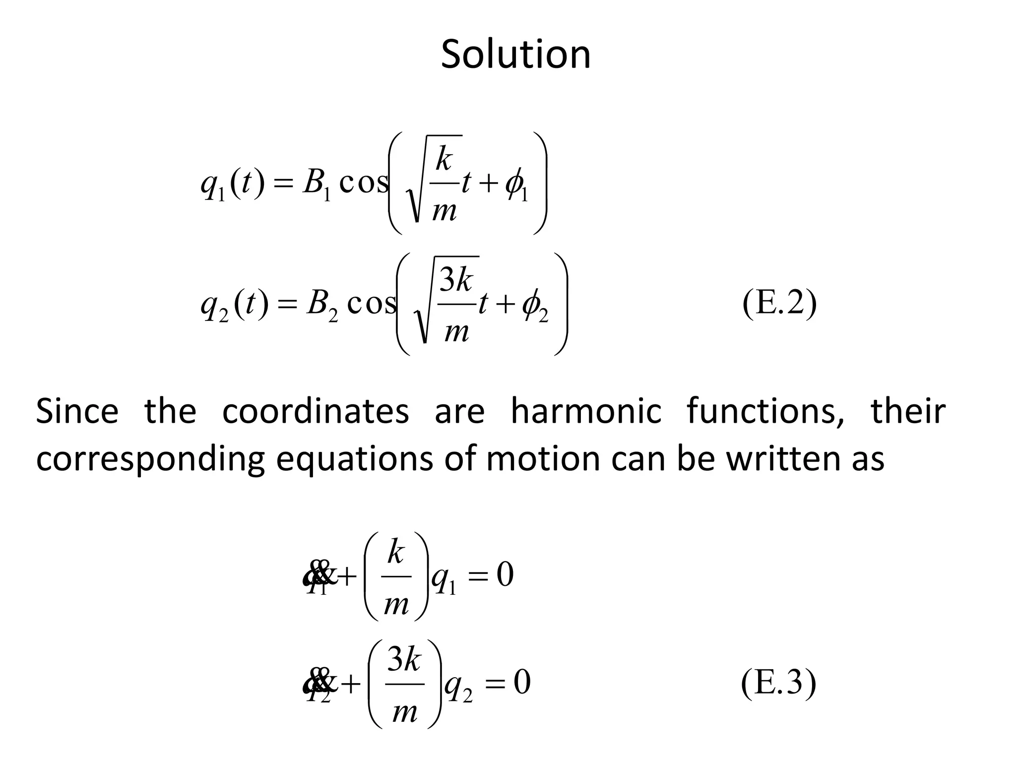
The solution of Eqs.(E.4) gives the principal coordinates:
From Eqs.(E.1) and (E.2), we can write
THANK YOU

two degree of freddom system

  • 1.
    GANDHINAGAR INSTITUTE OF TECHNOLOGY Subject:Dynamics of machine Topic:-Two degree of freedom system Branch:-Mechanical Sem.:-6 Div:-D Prepared By:- Guided By:- Patel Yash S. (150123119039) Prof. Samir Raval
  • 2.
    INTRODUCTION • The Systemwhich require two independent co-ordinates to specify its motion at configuration at instant is called two degree of freedom system. – Example: motor pump system. • There are two equations of motion for a 2DOF system, one for each mass (more precisely, for each DOF). • They are generally in the form of couple differential equation that is, each equation involves all the coordinates.
  • 3.
    Equation of motionfor forced vibration • Consider a viscously damped two degree of freedom spring-mass system, shown in Fig. Figure. A two degree of freedom spring-mass-damper system
  • 4.
    Equations of Motionfor Forced Vibration )2.5()()( )1.5()()( 2232122321222 1221212212111 Fxkkxkxccxcxm Fxkxkkxcxccxm     )3.5()()(][)(][)(][ tFtxktxctxm   Both equations can be written in matrix form as The application of Newton’s second law of motion to each of the masses gives the equations of motion: where [m], [c], and [k] are called the mass, damping, and stiffness matrices, respectively, and are given by
  • 5.
    Equations of Motionfor Forced Vibration                         322 221 322 221 2 1 ][ ][ 0 0 ][ kkk kkk k ccc ccc c m m m               )( )( )( )( )( )( 2 1 2 1 tF tF tF tx tx tx  And the displacement and force vectors are given respectively: It can be seen that the matrices [m], [c], and [k] are all 2 x 2 matrices whose elements are known masses, damping coefficient and stiffnesses of the system, respectively.
  • 6.
    Equations of Motionfor Forced Vibration ][][],[][],[][ kkccmm TTT  6 where the superscript T denotes the transpose of the matrix. oThe solution of Eqs.(5.1) and (5.2) involves four constants of integration (two for each equation). Usually the initial displacements and velocities of the two masses are specified as oFurther, these matrices can be seen to be symmetric, so that, x1(t = 0) = x1(0) and 1( t = 0) = 1(0), x2(t = 0) = x2(0) and 2 (t = 0) = 2(0). x x x x
  • 7.
    Free Vibration Analysisof an Undamped System )5.5(0)()()()( )4.5(0)()()()( 2321222 2212111   txkktxktxm txktxkktxm   )6.5()cos()( )cos()( 22 11     tXtx tXtx 7 Assuming that it is possible to have harmonic motion of m1 and m2 at the same frequency ω and the same phase angle Φ, we take the solutions as By setting F1(t) = F2(t) = 0, and damping disregarded, i.e., c1 = c2 = c3 = 0, and the equation of motion is reduced to:
  • 8.
    Free Vibration Analysisof an Undamped System       )7.5(0)cos()( 0)cos()( 232 2 212 22121 2 1     tXkkmXk tXkXkkm     )8.5(0)( 0)( 232 2 212 22121 2 1   XkkmXk XkXkkm   Since Eq.(5.7)must be satisfied for all values of the time t, the terms between brackets must be zero. Thus, Substituting into Eqs.(5.4) and (5.5),
  • 9.
    Free Vibration Analysisof an Undamped System     0 )( )( det 21 2 12 221 2 1            kkmk kkkm       )9.5(0))(( )()()( 2 23221 132221 4 21   kkkkk mkkmkkmm  or which represent two simultaneous homogenous algebraic equations in the unknown X1 and X2. For trivial solution, i.e., X1 = X2 = 0, there is no solution. For a nontrivial solution, the determinant of the coefficients of X1 and X2 must be zero:
  • 10.
    )10.5( ))(( 4 )()( 2 1 )()( 2 1 , 2/1 21 2 23221 2 21 132221 21 1322212 2 2 1                           mm kkkkk mm mkkmkk mm mkkmkk   The roots are called natural frequencies of the system. which is called the frequency or characteristic equation. Hence the roots are: FREE VIBRATION ANALYSIS OF AN UNDAMPED SYSTEM
  • 11.
    Free Vibration Analysisof an Undamped System )11.5( )( )( )( )( 32 2 22 2 2 21 2 21 )2( 1 )2( 2 2 32 2 12 2 2 21 2 11 )1( 1 )1( 2 1 kkm k k kkm X X r kkm k k kkm X X r             )12.5(and )2( 12 )2( 1 )2( 2 )2( 1)2( )1( 11 )1( 1 )1( 2 )1( 1)1(                                     Xr X X X X Xr X X X X  The normal modes of vibration corresponding to ω1 2 and ω2 2 can be expressed, respectively, as To determine the values of X1 and X2, given ratio which are known as the modal vectors of the system.
  • 12.
    Free Vibration Analysisof an Undamped System (5.17)modesecond )cos( )cos( )( )( )( modefirst )cos( )cos( )( )( )( 22 )2( 12 22 )2( 1 )2( 2 )2( 1)2( 11 )1( 11 11 )1( 1 )1( 2 )1( 1)1(                                               tXr tX tx tx tx tXr tX tx tx tx   0)0(,)0( ,0)0(constant,some)0( 2 )( 12 1 )( 11   txXrtx txXtx i i i   Where the constants , , and are determined by the initial conditions. The initial conditions are The free vibration solution or the motion in time can be expressed itself as )1( 1X )2( 1X 1 2
  • 13.
    Free Vibration Analysisof an Undamped System )14.5()()()( 2211 txctxctx   )15.5()cos()cos( )()()( )cos()cos()()()( 22 )2( 1211 )1( 11 )2( 2 )1( 22 22 )2( 111 )1( 1 )2( 1 )1( 11      tXrtXr txtxtx tXtXtxtxtx Thus the components of the vector can be expressed as The resulting motion can be obtained by a linear superposition of the two normal modes, Eq.(5.13) where the unknown constants can be determined from the initial conditions:
  • 14.
    Free Vibration Analysisof an Undamped System )16.5()0()0(),0()0( ),0()0(),0()0( 2222 1111 xtxxtx xtxxtx     )17.5(sinsin)0( coscos)0( sinsin)0( coscos)0( 2 )2( 1221 )1( 1112 2 )2( 121 )1( 112 2 )2( 121 )1( 111 2 )2( 11 )1( 11     XrXrx XrXrx XXx XXx                                           )( )0()0( sin, )( )0()0( sin )0()0( cos, )0()0( cos 122 211 2 )2( 1 121 212 1 )1( 1 12 211 2 )2( 1 12 212 1 )1( 1 rr xxr X rr xxr X rr xxr X rr xxr X       Substituting into Eq.(5.15) leads to The solution can be expressed as
  • 15.
    Free Vibration Analysisof an Undamped System                   )18.5( )0()0([ )0()0( tan cos sin tan )0()0([ )0()0( tan cos sin tan )0()0( )0()0( )( 1 sincos )0()0( )0()0( )( 1 sincos 2112 2111 2 )2( 1 2 )2( 11 2 2121 2121 1 )1( 1 1 )1( 11 1 2/1 2 2 2 2112 211 12 2/12 2 )2( 1 2 2 )2( 1 )2( 1 2/1 2 1 2 2122 212 12 2/12 1 )1( 1 2 1 )1( 1 )1( 1                                                         xxr xxr X X xxr xxr X X xxr xxr rr XXX xxr xxr rr XXX               from which we obtain the desired solution
  • 16.
    Example :Free VibrationResponse of a Two Degree of Freedom System ).0()0()0(,1)0( 2211 xxxx   (E.1) 0 0 55- 53510 0 0 2 1 2 2 2 1 32 2 22 221 2 1                                               X X X X kkmk kkkm     Solution: For the given data, the eigenvalue problem, Eq.(5.8), becomes Find the free vibration response of the system shown in Fig.5.3(a) with k1 = 30, k2 = 5, k3 = 0, m1 = 10, m2 = 1 and c1 = c2 = c3 = 0 for the initial conditions or
  • 17.
  • 18.
  • 19.
    Solution (E.12) 7 2 cos; 7 5 cos 2 )2( 11 )1( 1  XX (E.13)0sin,0sin 2 )2( 11 )1( 1   XX (E.14)0,0, 7 2 , 7 5 21 )2( 1 )1( 1  XX while the solution of Eqs.(E.10) and (E.11) leads to The solution of Eqs.(E.8) and (E.9) yields Equations (E.12) and (E.13) give
  • 20.
  • 21.
    Torsional System Figure :Torsional system with discs mounted on a shaft Consider a torsional system as shown in Fig. The differential equations of rotational motion for the discs can be derived as
  • 22.
    Torsional System 22312222 11221111 )( )( ttt ttt MkkJ MkkJ       )19.5()( )( 22321222 12212111 tttt tttt MkkkJ MkkkJ       which uponrearrangement become For the free vibration analysis of the system, Eq.(5.19) reduces to )20.5(0)( 0)( 2321222 2212111     ttt ttt kkkJ kkkJ  
  • 23.
    Coordinate Coupling andPrincipal Coordinates Generalized coordinates are sets of n coordinates used to describe the configuration of the system. •Equations of motion Using x(t) and θ(t).
  • 24.
    Coordinate Coupling andPrincipal Coordinates )21.5()()( 2211  lxklxkxm  )22.5()()( 2221110 llxkllxkJ   and the moment equation about C.G. can be expressed as From the free-body diagram shown in Fig.5.10a, with the positive values of the motion variables as indicated, the force equilibrium equation in the vertical direction can be written as Eqs.(5.21) and (5.22) can be rearranged and written in matrix form as
  • 25.
    Coordinate Coupling andPrincipal Coordinates )23.5( 0 0 )()( )()( 0 0 2 2 2 12211 221121 0 21                                      x lklklklk lklkkkx J m     melyklykym  )()( 2211 The lathe rotates in the vertical plane and has vertical motion as well, unless k1l1 = k2l2. This is known as elastic or static coupling. From Fig.5.10b, the equations of motion for translation and rotation can be written as •Equations of motion Using y(t) and θ(t).
  • 26.
    Coordinate Coupling andPrincipal Coordinates )24.5()()( 222111 ymellykllykJP    )25.5( 0 0 )()( )()( 2 2 2 112211 112221 2                                      y lklklklk lklkkky Jme mem P   2211 lklk  These equations can be rearranged and written in matrix form as If , the system will have dynamic or inertia coupling only. Note the following characteristics of these systems:
  • 27.
    Coordinate Coupling andPrincipal Coordinates )26.5( 0 0 2 1 2221 1211 2 1 2221 1211 2 1 2221 1211                                              x x kk kk x x cc cc x x mm mm     1. In the most general case, a viscously damped two degree of freedom system has the equations of motions in the form: 2. The system vibrates in its own natural way regardless of the coordinates used. The choice of the coordinates is a mere convenience. 3. Principal or natural coordinates are defined as system of coordinates which give equations of motion that are uncoupled both statically and dynamically.
  • 28.
    Example :Principal Coordinatesof Spring-Mass System Determine the principal coordinates for the spring-mass system shown in Fig.
  • 29.
    Solution (E.1) 3 coscos)( 3 coscos)( 22112 22111                                     t m k Bt m k Btx t m k Bt m k Btx We define anew set of coordinates such that Approach: Define two independent solutions as principal coordinates and express them in terms of the solutions x1(t) and x2(t). The general motion of the system shown is
  • 30.
  • 31.
  • 32.