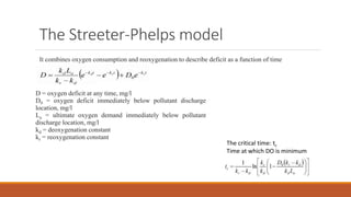
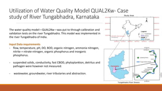
This document provides an overview of mathematical modelling of streams. It discusses the need for modelling to simulate different water quality scenarios and management strategies. It introduces various types of mathematical models and describes the governing laws and equations used in water quality models. Key aspects covered include modelling of dissolved oxygen levels using the Streeter-Phelps model, and a case study applying the QUAL2Kw model to a river in Karnataka, India.

1. Mathematical modelling
of streams

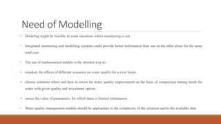
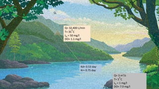
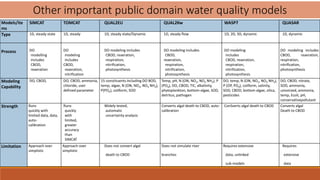
2. Table of Contents
Introduction
Need of Modelling
Mathematical modelling - The Introduction
Mathematical modelling - Process and Types
Water quality modeling - Basics
Water quality modeling - Governing Laws & Equations
Water quality modeling - Transport in Streams and canals
Modelling of Dissolved oxygen
The Streeter-Phelps model & application
Case study- QUAL2Kw Model

3. Introduction
• Water quality management is a critical component of overall integrated water resources management.
• All living organisms require water of sufficient quantity and quality to survive, although different aquatic species
can tolerate different levels of water quality.
• Modelling is a continuous process of developing models in times parallel with the increase of the available
information and knowledge about the simulation system, which more and more adequate to describe the
real process.
• The models available to help managers predict water quality impacts are relatively simple compared with the
complexities of actual water systems.
• Modelling can be used to assess (predict) future water quality situations resulting from different management
strategies.

4. Need of Modelling
• Modeling might be feasible in some situations where monitoring is not.
• Integrated monitoring and modelling systems could provide better information than one or the other alone for the same
total cost.
• The use of mathematical models is the shortest way to:
 simulate the effects of different scenarios on water quality for a river basin;
 choose solutions where and how to invest for water quality improvement on the basis of comparison among needs for
water with given quality and investment option;
 assess the value of parameters, for which there is limited information.
• Water quality management models should be appropriate to the complexity of the situation and to the available data

5. Mathematical modelling
Study the real world problems in mathematical terms
Conversion of physical situations into mathematical terms using suitable
conditions and variables
To project how the system/ conditions will change over a period of time
and in response to manipulation
A mathematical model is only a complement and do not replace the
theory and experimentation in scientific research
What
How
Why

6. Process and Types
a. Discrete Continuous
b. Static Dynamic
c. Linear Non Linear
d. Deterministic Probabilistic
e. Qualitative Quantitative
f. Explicit Implicit
Real world
problem
Result
Computational
model
Mathematical
model
Working model
Translate
Simplify
Interpret
Simulate
Represent

7. Governing Laws
1. Conservation of Mass: Mass balance in a CV
Density ƿ = ƿ(x,y,z,t) velocity v= v(x,y,z,t):
Mass
Momentum
Heat/ energy
2. Conservation of momentum- Navier strokes equation

8. Water quality models
•Water quality models simulate the fate of pollutants &
state of water quality variables in water bodies
•Incorporates variety of physical, chemical, & biological
processes which control the transport and transformation
of these variables.
•Temperature, solar radiation, wind speed, pH, and light
attenuation coefficients – Important components
•Each water quality model has its own set of characteristics
and requirements- ( some models can be applied to several
types of water bodies and some models only for particular
water bodies)

9. Water Quality Modeling
A typical water quality model consists of a collection of formulations
representing physical mechanisms that determine position and
momentum of pollutants in a water body.
i. Advective transport formulations;
ii. Dispersive transport formulation;
iii. Dissolved oxygen saturation;
iv. Carbonaceous deoxygenation, Sediment, BOD, pH, Alkalinity,
Nutrients, Algae, Microorganism, etc.
Substances
Particle
Dissolved Emulsified
1. Hydrodynamically
neutral
2. Hydrodynamically
active
1. Bed rock material
2. Sediments
1. Drops
2. Bubbles

10. The transport of pollutants in water body is through
1. Diffusive processes
2. Turbulent flow
• Mass transport equation
• Heat transfer equation
 Fick’s law:
Specific mass flux
3. Conservation of Heat / Energy

11. Transport in Streams and canals
One dimensional transport equation
Two dimensional transport equation
Three dimensional transport equation
• Vx = mean velocity in x direction
• Vy = mean velocity in y direction
• Vz = mean velocity in z direction
• C= concentration of pollutant over
the cross sectional area
• I = sink or source term (reaction of
substance with its environment)
• K= dispersion coefficient

12. Surface water quality: Rivers & Streams
Surface water bodies
•Highly susceptible to contamination
•Source of majority of our waters
•Organic and oxygen consuming waste constitutes the most significant part of the pollution load.
•Principle water quality problem associated with these waters is the depletion in DO content
Sinks of DO in Rivers
 Oxidation of carbonaceous waste material
 Oxidation of nitrogenous wastes
 Oxygen demand of sediment (SOD)
 Use of O2 for respiration of aquatic plants
Sources of DO in Rivers
 Reaeration from atmosphere
 Photosynthetic O2 production
 Do in incoming tributaries or effluents

13. Modelling of Dissolved oxygen
The classic stream dissolved oxygen modeling has been attributed to Streeter-Phelps equations, which
determines the relation between the dissolved oxygen concentration and the biological oxygen
demand over time and is a solution to the linear first order differential equation.
The key model assumptions are:
 Continuous discharge of waste at a given
location
 Uniform mixing of river water and wastewater
 No dispersion of waste in the direction of
flow (i.e, plug flow assumed)
Two key processes
considered:
 Source of DO: Reaeration from
atmosphere
 Sink of DO: Oxidation of organic matter
(carbonaceous)

15. The Oxygen sag curve
Deficit (D)
Dissolved Oxygen (DO)
DO min
Saturation D0
Initial deficit, D0
Critical point
Oxygen deficit
The measure of where the saturation concentration
of DO is and where it should ideally be
DO deficit = Saturation Conc. – Actual Conc.
Microbes in the stream consume substrate according
to the first order kinetics ,
Kd= Deoxygenation rate constant (O2 consumption)
Kr= Reoxygenation rate constant (O2 replenishment)

16. Oxygen balance
Rate of Oxygen
accumulating
Rate of oxygen
in
Rate of oxygen
out
Rate of oxygen
produced
Rate of oxygen
consumed
Considering a swift stream,
The rate of production of Oxygen will be negligible
The water is below saturation so no Oxygen concentration out
ⅆ𝑐
dt
Rate of oxygen
in
Rate of oxygen
consumed

17. The Streeter-Phelps model
It combines oxygen consumption and reoxygenation to describe deficit as a function of time
D = oxygen deficit at any time, mg/l
D0 = oxygen deficit immediately below pollutant discharge
location, mg/l
La = ultimate oxygen demand immediately below pollutant
discharge location, mg/l
kd = deoxygenation constant
kr = reoxygenation constant
The critical time: tc
Time at which DO is minimum

18. Q.
Q= 3 m3/s
T= 5 ͦͦC
L0 = 1 mg/l
DO= 7.0 mg/l
Q= 32,400 L/min
T= 35 ͦͦC
L0 = 50 mg/l
DO= 1.1 mg/l
Kd= 0.53 day-
Kr= 0.75 day-

19. Q1 What will be the temperature of mixed water ?
T3 = T1Q1 + T2Q2 = (5 ͦͦC)(3 m3/s)+(35 ͦͦC)(0.54m3/s) = 9.6 ͦͦC = 10 ͦͦC
Q3 3.54 m3/s
Q2 What is the DO concentration of mixed water ?
D3 = D1Q1 + D2Q2 = (7.0 mg/l )(3 m3/s)+(1.1 mg/l )(0.54m3/s) = 6.1mg/l
Q3 3.54 m3/s
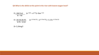
Q3 What is the time to the critical point of lowest Dissolved oxygen ?
= 1 ln [ 0.75 x (1- 5.17 (0.75-0.53)] = 0.25 day
(0.75-0.53) 0.53 0.53x 8.47

20. Q4 What is the deficit at the point in the river with lowest oxygen level?
D = (kd) (La) (e (-kdt) – e(-krt))+ Doe (-krt)
kr – kd
D = (0.53) (8.47) (e (-0.53x0.25) – e(-0.75x0.25)) = 5.17e (-0.75x0.25)
0.75 – 0.53
D= 5.24mg/l

21. Utilization of Water Quality Model QUAL2Kw- Case
study of River Tungabhadra, Karnataka
The water quality model—QUAL2Kw—was put to through calibration and
validation tests on the river Tungabhadra. This model was implemented in
the river Tungabhadra of India.
Input Data requirements
- flow, temperature, pH, DO, BOD, organic nitrogen, ammonia nitrogen,
nitrite + nitrate nitrogen, organic phosphorus and inorganic
phosphorus.
- suspended solids, conductivity, fast CBOD, phytoplankton, detritus and
pathogen were however not measured.
- wastewater, groundwater, river tributaries and abstraction.

22. Model Parameters
The ranges of model rate parameters were obtained from Environmental Protection
Agency (EPA) guidance document, QUAL2Kw user manual and Documentation for the
enhanced stream water quality model QUAL2E and QUAL2E-UNCAS.
QUAL2Kw has eight options to calculate re-aeration rate as a function of the river
hydraulics. Owens-Gibbs formula was used , which was developed for streams exhibiting
depths ranging from 0.4 to 11 feet and velocities ranging from 0.1 to 5 feet/s
Conclusion
• The modelling was done on the basis of following water quality control techniques
- flow augmentation, local oxygenation and pollution loads modification.
• Local oxygenation is effective in raising dissolved oxygen levels.
• A combination of wastewater modification, flow augmentation and local oxygenation
can be used to ensure the requirements for the minimum DO concentrations are met.
• The model has many advantages and can be used as a top choice when thinking of
river water policy options.
Mass balance equation in
reach segment

23. Models/ite
ms
SIMCAT TOMCAT QUAL2EU QUAL2Kw WASP7 QUASAR
Type 1D, steady state 1D, steady 1D, steady state/Dynamic 1D, steady flow 1D, 2D, 3D, dynamic 1D, dynamic
Process DO
modelling
includes
CBOD,
reaeration
DO
modeling
includes
CBOD,
reaeration,
nitrification
DO modeling includes
CBOD, reaeration,
respiration,
nitrification,
photosynthesis
DO modeling includes
CBOD,
reaeration,
respiration,
nitrification,
photosynthesis
DO modeling
includes
CBOD, reaeration,
respiration,
nitrification,
photosynthesis
DO modeling includes
CBOD, reaeration,
respiration,
nitrification,
photosynthesis
Modeling
Capability
DO, CBOD, DO, CBOD, ammonia,
chloride, user
defined parameter
15 constituents including DO BOD,
temp, algae, N (ON, NO2, NO3 NH3),
P(PO4), coliform, SOD
Temp, pH, N (ON, NO2, NO3 NH3), P
(PO4), DO, CBOD, TIC, alkalinity,
phytoplankton, bottom-algae, SOD,
detritus, pathogen
DO, temp, N (ON, NO2, NO3 NH3),
P (OP, PO4), coliform, salinity,
SOD, CBOD, bottom algae, silica,
pesticides
DO, CBOD, nitrate,
SOD, ammonia,
unionized, ammonia,
temp, Ecoli, pH,
conservativepollutant
Strength Runs
quickly with
limited data, data,
auto-
calibration
Runs
quickly
with
limited,
greater
accuracy
than
SIMCAT
Widely tested,
automatic
uncertainty analysis
Converts algal death to CBOD, auto-
calibration
ConSverts algal death to CBOD Converts algal
Death to CBOD
Limitation Approach over
simplistic
Approach over
simplistic
Does not convert algal
death to CBOD
Does not simulate river
branches
Requires extensive
data, unlinked
sub-models
Requires
extensive
data
Other important public domain water quality models