LECTURE SERIES
Dep. of Geography,
Yogyakarta State
University
Dr SRI ADIYANTI
School of Earth &
Environment,
Fac. of Science UWA
LECTURE DAY-4
Introduction to Lake
Hydrodynamic Water Quality
Modelling
DAY 1: ENVIRONMENTAL HYDROLOGY
 Introduction: Environmental Hydrology
 Water Balance
 Rainfall Spatio-temporal Variability
DAY 2: LINKAGE CATCHMENT-RIVER-ESTUARINE-OCEAN
 Case Study: Caboolture River Basin in Queensland
DAY 3: FIELD EXCURSION – WADUK SERMO
DAY 4:
A : INTRODUCTION TO LAKE HYDRODYNAMIC WATER QUALITY
MODELLING: Case Study Waduk Sermo & Group Presentation
B : HOW TO GET SCHOLARSHIP & WORK PROFESSIONALLY OVERSEAS
AGENDA: 3-DAY LECTURE + EXCURSION
WHY DO WE NEED A
WATER QUALITY MODEL ?
Water Quality Models as
‘Virtual Environmental Laboratories’
• Reconcile theory with observation
• Improve system understanding:
– Quantify processes and controls on variability
– Risk assessments
– Conduct system budgets (eg. nutrients, metals)
– System feedbacks & non-linearity
• Assess management interventions (eg. scenarios):
– Flushing/diversions
– Chemical amelioration or bio-manipulation
– Engineering interventions (pumping; destratification)
• Real-time prediction:
– Water quality alerts & risk assessment
– Fore-casting
The problem we need to solve
light salinity
phytoplankton
zooplankton
CO2NO3
-
PO4
2-
O2
fish
bacteria
detritus
temperature
Management questions …
• How are the regulated/assimilated once they enter
surface waters?
– Physical (hydrodynamic) vs ecological controls
• How do changes in catchment nutrient export manifest
in water bodies?
• Can we unravel this complexity to improve science-
basis of load targets?
The modelling process
• Defining your domain
– For GLM: Height-Storage relationship (Bathymetry)
• Define what is being simulated:
– Identify state variables (temperature, salinity, nutrients?)
– What is the grid resolution & time-step
• Connecting to the external environment:
– Setting boundary conditions:
• Inflows (flow, temp, salinity, wq attrobutes)
• Meteorology
• Getting ready to start: providing an initial condition
WHAT TYPE OF MODEL
SHOULD WE USE?
Empirical models of water quality
response ….
• Vollenweider and statistical relationships
Control
+P
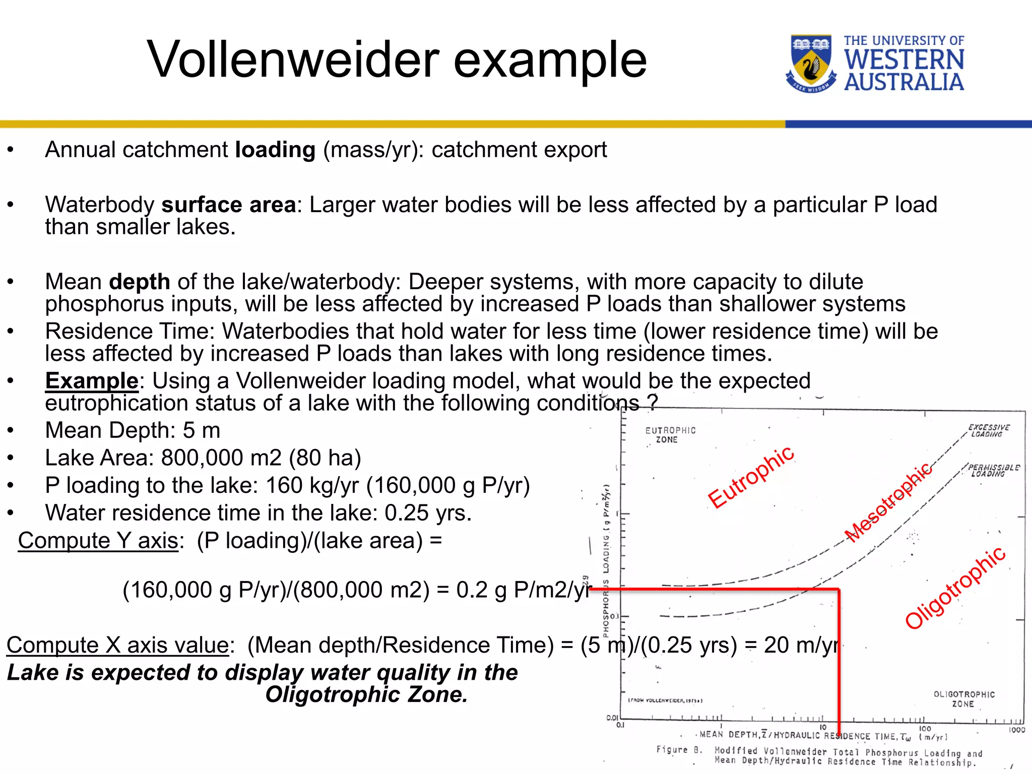
Vollenweider example
• Annual catchment loading (mass/yr): catchment export
• Waterbody surface area: Larger water bodies will be less affected by a particular P load
than smaller lakes.
• Mean depth of the lake/waterbody: Deeper systems, with more capacity to dilute
phosphorus inputs, will be less affected by increased P loads than shallower systems
• Residence Time: Waterbodies that hold water for less time (lower residence time) will be
less affected by increased P loads than lakes with long residence times. 

• Example: Using a Vollenweider loading model, what would be the expected
eutrophication status of a lake with the following conditions ? 

• Mean Depth: 5 m
• Lake Area: 800,000 m2 (80 ha)
• P loading to the lake: 160 kg/yr (160,000 g P/yr)
• Water residence time in the lake: 0.25 yrs.

Compute Y axis:
(P loading)/(lake area) =
(160,000 g P/yr)/(800,000 m2) = 0.2 g P/m2/yr
Compute X axis value:
(Mean depth/Residence Time) = (5 m)/(0.25 yrs) = 20 m/yr 

Lake is expected to display water quality in the
Oligotrophic Zone.
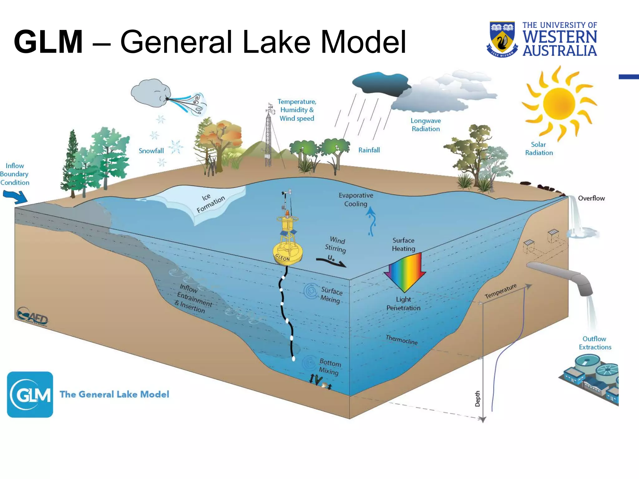
GLM – General Lake Model
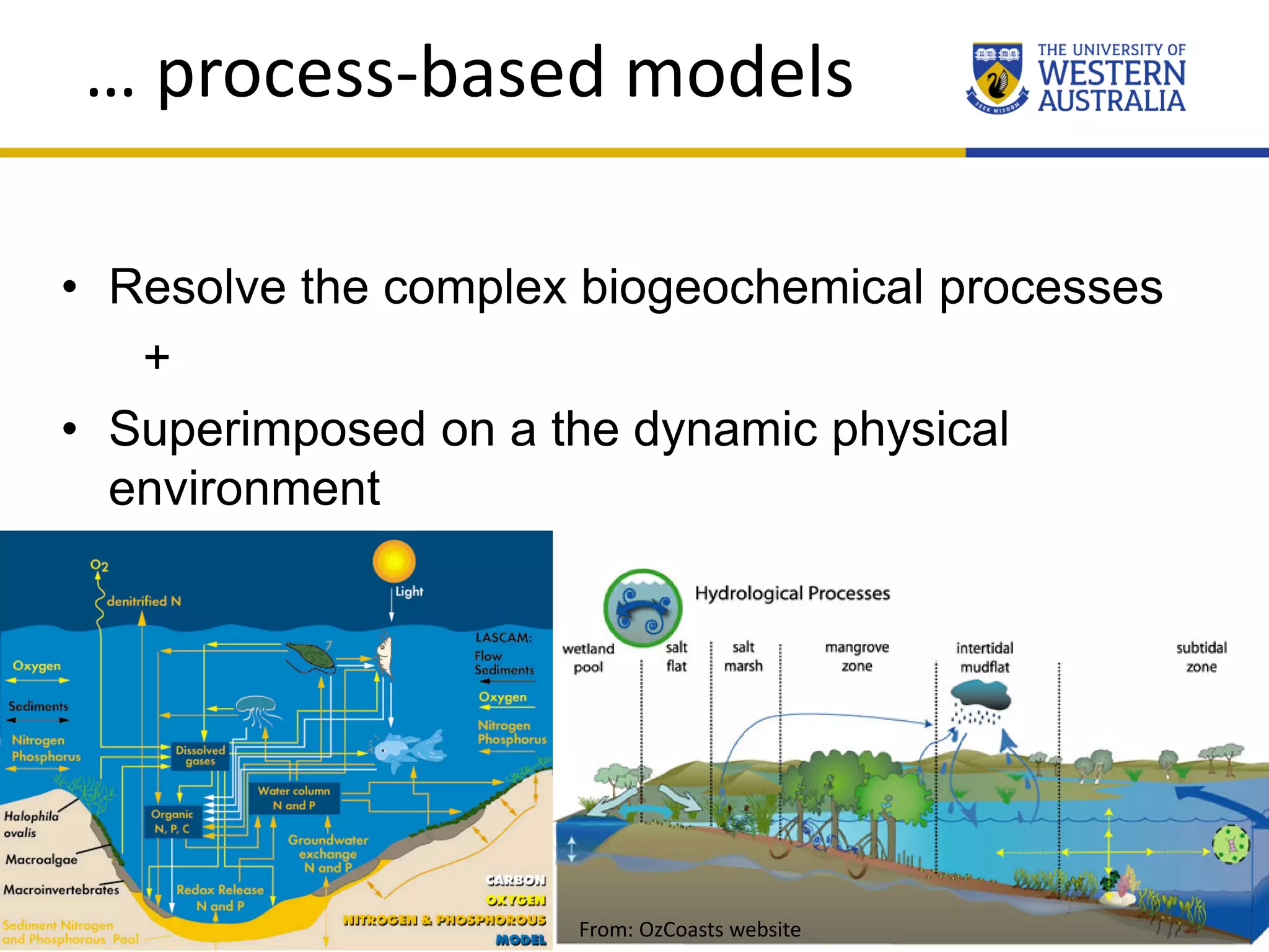
… process-based models
• Resolve the complex biogeochemical processes
+
• Superimposed on a the dynamic physical
environment
From: OzCoasts website
Model Dimension
• 0D – mixed ‘container’, one grid box
– Assumes the lake is a ‘bathtub’, ie, homogenous conditions
• 1D – a single dimension is resolved
– rivers: narrow and shallow river, row of grid cells
– lakes: layers of cells to resolve vertical stratification
• 2D – shallow lake or coastal lagoon,
2D matrix of grid cells
(can be vertically averaged or laterally averaged)
• 3D – wide and deep river, lake or coastal area with
vertical stratification, usually a 3D matrix of grid cells
Basic idea of numerical modeling
t
1) Divide area into smaller sub-areas (grid cells)
2) Solve flow and other processes in each grid cell
3) Connect grid cells through transport, diffusion and
other processes
Connection between grid cells
Qin Qout
Qw
Horizontal (left) and vertical (right, Qw) transport between
grid cells
• Conservation of Mass
• Control volume in changes reflect inputs and outputs
• Includes inflows/withdrawals
• Conservation of Momentum
• Velocity based on balances of forces
• Bed slope, elevation differences (gravity)
• Depth gradient (pressure slope)
• Friction (based on drag with bed / vegetation etc)
• Rotation of earth for large domains (coriolis)
Physical Basis
Basis for flow and transport models
TUFLOW-FV – www.tuflow.com
Finite volume – complex environments
Connecting our domain to the
surrounding environment
Modelling Lake Stratification
surface mixingsurface fluxes
artificial
destratification
1D – laterally averaged models: assume most variability is vertical
The General Lake Model (GLM
Tdensity
InflowSurface fluxes
mixing
Model Inputs:
• Discharges: Inflow & Outflow
• Meteorology: solar radiation, long-wave radiation, air temperature, wind
speed and direction, humidity
CASE STUDY: WADUK SERMO, Kulon Progo
• Temperature profiles
• pH Profiles
• Dissolved Oxygen profiles
For validation:
Waduk Sermo
Waduk Sermo
Lake Water Balance Component
INFLOW
OUTFLOW
EVAPORATION
RAINFALL
Bathymetry (Area-Storage-Elevation
Relationship) / Kurva Karasteristik
GROUP I: WATER BALANCE
GROUP II: OUTFLOW DISCHARGE MEASUREMENT
GROUP III: PHYSICO-CHEMICAL PROPERTY
MEASUREMENT
GROUP PRESENTATION:

WATER QUALITY MODELING DR. YANTI

  • 1.
    LECTURE SERIES Dep. ofGeography, Yogyakarta State University Dr SRI ADIYANTI School of Earth & Environment, Fac. of Science UWA LECTURE DAY-4 Introduction to Lake Hydrodynamic Water Quality Modelling
  • 2.
    DAY 1: ENVIRONMENTALHYDROLOGY  Introduction: Environmental Hydrology  Water Balance  Rainfall Spatio-temporal Variability DAY 2: LINKAGE CATCHMENT-RIVER-ESTUARINE-OCEAN  Case Study: Caboolture River Basin in Queensland DAY 3: FIELD EXCURSION – WADUK SERMO DAY 4: A : INTRODUCTION TO LAKE HYDRODYNAMIC WATER QUALITY MODELLING: Case Study Waduk Sermo & Group Presentation B : HOW TO GET SCHOLARSHIP & WORK PROFESSIONALLY OVERSEAS AGENDA: 3-DAY LECTURE + EXCURSION
  • 3.
    WHY DO WENEED A WATER QUALITY MODEL ?
  • 4.
    Water Quality Modelsas ‘Virtual Environmental Laboratories’ • Reconcile theory with observation • Improve system understanding: – Quantify processes and controls on variability – Risk assessments – Conduct system budgets (eg. nutrients, metals) – System feedbacks & non-linearity • Assess management interventions (eg. scenarios): – Flushing/diversions – Chemical amelioration or bio-manipulation – Engineering interventions (pumping; destratification) • Real-time prediction: – Water quality alerts & risk assessment – Fore-casting
  • 5.
    The problem weneed to solve light salinity phytoplankton zooplankton CO2NO3 - PO4 2- O2 fish bacteria detritus temperature
  • 6.
    Management questions … •How are the regulated/assimilated once they enter surface waters? – Physical (hydrodynamic) vs ecological controls • How do changes in catchment nutrient export manifest in water bodies? • Can we unravel this complexity to improve science- basis of load targets?
  • 7.
    The modelling process •Defining your domain – For GLM: Height-Storage relationship (Bathymetry) • Define what is being simulated: – Identify state variables (temperature, salinity, nutrients?) – What is the grid resolution & time-step • Connecting to the external environment: – Setting boundary conditions: • Inflows (flow, temp, salinity, wq attrobutes) • Meteorology • Getting ready to start: providing an initial condition
  • 8.
    WHAT TYPE OFMODEL SHOULD WE USE?
  • 9.
    Empirical models ofwater quality response …. • Vollenweider and statistical relationships Control +P
  • 10.
    Vollenweider example • Annualcatchment loading (mass/yr): catchment export • Waterbody surface area: Larger water bodies will be less affected by a particular P load than smaller lakes. • Mean depth of the lake/waterbody: Deeper systems, with more capacity to dilute phosphorus inputs, will be less affected by increased P loads than shallower systems • Residence Time: Waterbodies that hold water for less time (lower residence time) will be less affected by increased P loads than lakes with long residence times. 
 • Example: Using a Vollenweider loading model, what would be the expected eutrophication status of a lake with the following conditions ? 
 • Mean Depth: 5 m • Lake Area: 800,000 m2 (80 ha) • P loading to the lake: 160 kg/yr (160,000 g P/yr) • Water residence time in the lake: 0.25 yrs. 
Compute Y axis:
(P loading)/(lake area) = (160,000 g P/yr)/(800,000 m2) = 0.2 g P/m2/yr Compute X axis value:
(Mean depth/Residence Time) = (5 m)/(0.25 yrs) = 20 m/yr 
 Lake is expected to display water quality in the Oligotrophic Zone.
  • 11.
    GLM – GeneralLake Model
  • 12.
    … process-based models •Resolve the complex biogeochemical processes + • Superimposed on a the dynamic physical environment From: OzCoasts website
  • 13.
    Model Dimension • 0D– mixed ‘container’, one grid box – Assumes the lake is a ‘bathtub’, ie, homogenous conditions • 1D – a single dimension is resolved – rivers: narrow and shallow river, row of grid cells – lakes: layers of cells to resolve vertical stratification • 2D – shallow lake or coastal lagoon, 2D matrix of grid cells (can be vertically averaged or laterally averaged) • 3D – wide and deep river, lake or coastal area with vertical stratification, usually a 3D matrix of grid cells
  • 14.
    Basic idea ofnumerical modeling t 1) Divide area into smaller sub-areas (grid cells) 2) Solve flow and other processes in each grid cell 3) Connect grid cells through transport, diffusion and other processes
  • 15.
    Connection between gridcells Qin Qout Qw Horizontal (left) and vertical (right, Qw) transport between grid cells
  • 16.
    • Conservation ofMass • Control volume in changes reflect inputs and outputs • Includes inflows/withdrawals • Conservation of Momentum • Velocity based on balances of forces • Bed slope, elevation differences (gravity) • Depth gradient (pressure slope) • Friction (based on drag with bed / vegetation etc) • Rotation of earth for large domains (coriolis) Physical Basis Basis for flow and transport models
  • 18.
    TUFLOW-FV – www.tuflow.com Finitevolume – complex environments
  • 19.
    Connecting our domainto the surrounding environment
  • 20.
    Modelling Lake Stratification surfacemixingsurface fluxes artificial destratification 1D – laterally averaged models: assume most variability is vertical
  • 21.
    The General LakeModel (GLM Tdensity InflowSurface fluxes mixing
  • 23.
    Model Inputs: • Discharges:Inflow & Outflow • Meteorology: solar radiation, long-wave radiation, air temperature, wind speed and direction, humidity CASE STUDY: WADUK SERMO, Kulon Progo • Temperature profiles • pH Profiles • Dissolved Oxygen profiles For validation:
  • 24.
  • 25.
  • 26.
    Lake Water BalanceComponent INFLOW OUTFLOW EVAPORATION RAINFALL
  • 27.
  • 28.
    GROUP I: WATERBALANCE GROUP II: OUTFLOW DISCHARGE MEASUREMENT GROUP III: PHYSICO-CHEMICAL PROPERTY MEASUREMENT GROUP PRESENTATION: