This document provides information about the Engineering Mathematics-I course MAT 1151 including:
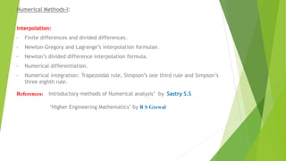
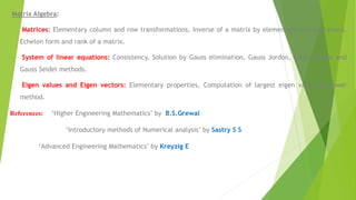
- Details about the course structure over two semesters covering topics like matrix algebra, linear algebra, differential equations, and numerical methods.
- Lists of chapters and topics to be covered in each semester along with references for further reading.
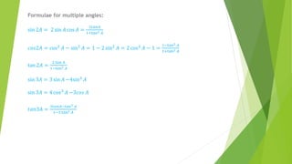
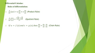
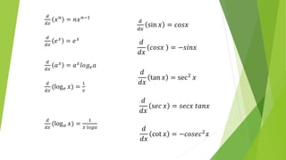
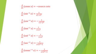
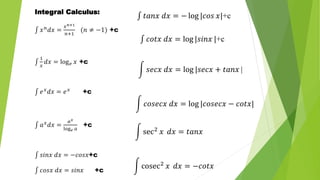
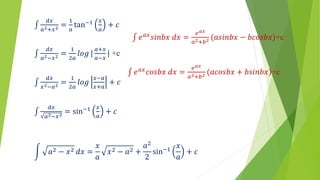
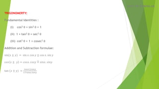
- Formulas from trigonometry, linear algebra, differential calculus, and integral calculus that will be useful for the course.

![Transforming product into sum :
sin x. cos y = ½ [sin (x + y) + sin (x – y)] cos x. sin y = ½ [sin (x + y) – sin (x – y)]
cos x. cos y = ½ [cos (x + y) + cos (x – y)] sin x. sin y = ½ [cos (x – y) – cos (x + y)]
Transforming sum into product:
sin 𝐶 + sin 𝐷 = 2 sin
𝐶+𝐷
2
𝑐𝑜𝑠
𝐶−𝐷
2
sin 𝐶 − sin 𝐷 = 2 cos
𝐶+𝐷
2
𝑠𝑖𝑛
𝐶−𝐷
2
cos 𝐶 + cos 𝐷 = 2 cos
𝐶+𝐷
2
𝑐𝑜𝑠
𝐶−𝐷
2
cos 𝐶 − 𝑐𝑜𝑠 𝐷 = −2 sin
𝐶+𝐷
2
𝑠𝑖𝑛
𝐶−𝐷
2](https://image.slidesharecdn.com/mathppt-240313162110-d958277a/85/Math-ppt-pptx-9-320.jpg)