1. The document discusses queueing theory and the M/M/1 queue model. The M/M/1 queue refers to a single server queue where inter-arrival times and service times are exponentially distributed. 2. It provides the equations that define the steady-state probabilities (Pn) for each number of customers (n) in the M/M/1 queue. These equations balance the rates of entering and leaving each state. 3. The limiting probabilities are then used to calculate key metrics like the average number of customers in the system (L) and average wait time (W).

1. meu = Service Rate = departure rate, also
in single server model
see next page example
unit (example: 12 customers/sec)
Short Q:
Applications of Queueing Theory:
Queueing theory has many
real world applications in algorithm
design and analysis, Network design,
Network performance optimization & analysis,
Network device design
(e.g., customers mimic the random arrival
of data packets from the network in the
Modem's data buffer/queue, gets service
by the CPU, thus CPU = server,
Data packets from Network = Customer
Modem's data buffer = Queue)
Markovian means "discrete time". No two events are
simultaneous. No two customers can arrive/depart
at the exact same moment
Memoryless => As arrival times poisson distributed, this implies
inter-arrival time exponentially distributed
(Exponential distribution ihas
memoryless property)
(service time
exponentially
distributed)
On average, (random, probabilistic
NOT every second the
same service time or rate)
***M/M/1 queue is
also called
Single Server
Exponential Queue
if n=3 (i.e., 3 servers)
then>>
at present L = 8
Lq = 5
(L = no of customers
in the system
Lq = no of customers
waiting in QueueQueue
Single Server
Exponential
Queueing
System
OR M/M/1
Queue Model

2. Just an example of random arrivals and how queue forms as 15, 22, 12 all >= 12 (i.e., service rate):
But,Probabilistic & Random,
NOT every minute gets exactly 10
cusomers!! See following example ...
Similarly: M/G/1 queue system: Markovian+General+single server:
Markovian events, Customer Arrivals follow any General probability distribution,
and the queueing system has only a single server (hence the '1' in M/G/1)
M/G/k: Markovian General queueing system with k servers
M/M/k : Markovian Memoryless queueing system with k servers
M: Markovian (discrete time) system G: The arrival of customers follw some General probability
distribution (instead of Poisson o exponential distribution) k: no. of servers is k
Example:
0

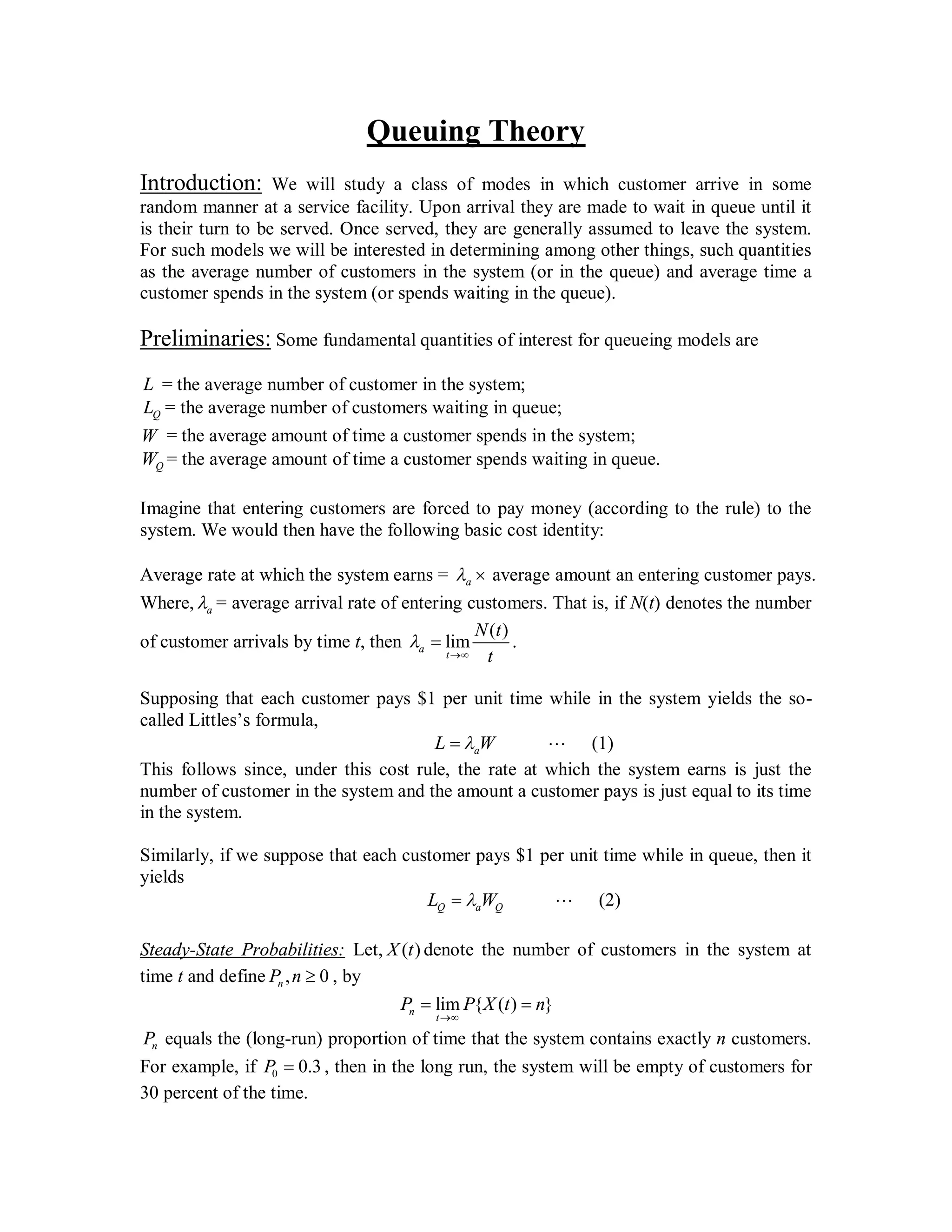
3. Queuing Theory
Introduction: We will study a class of modes in which customer arrive in some
random manner at a service facility. Upon arrival they are made to wait in queue until it
is their turn to be served. Once served, they are generally assumed to leave the system.
For such models we will be interested in determining among other things, such quantities
as the average number of customers in the system (or in the queue) and average time a
customer spends in the system (or spends waiting in the queue).
Preliminaries: Some fundamental quantities of interest for queueing models are
L = the average number of customer in the system;
QL = the average number of customers waiting in queue;
W = the average amount of time a customer spends in the system;
QW = the average amount of time a customer spends waiting in queue.
Imagine that entering customers are forced to pay money (according to the rule) to the
system. We would then have the following basic cost identity:
Average rate at which the system earns = a  average amount an entering customer pays.
Where, a = average arrival rate of entering customers. That is, if N(t) denotes the number
of customer arrivals by time t, then
( )
lima
t
N t
t


 .
Supposing that each customer pays $1 per unit time while in the system yields the so-
called Littles’s formula,
aL W  (1)
This follows since, under this cost rule, the rate at which the system earns is just the
number of customer in the system and the amount a customer pays is just equal to its time
in the system.
Similarly, if we suppose that each customer pays $1 per unit time while in queue, then it
yields
Q a QL W  (2)
Steady-State Probabilities: Let, ( )X t denote the number of customers in the system at
time t and define , 0nP n  , by
lim { ( ) }n
t
P P X t n

 
nP equals the (long-run) proportion of time that the system contains exactly n customers.
For example, if 0 0.3P  , then in the long run, the system will be empty of customers for
30 percent of the time.
L = (lambda) * W, Suppose you are waiting for 10 sec, on average 5 customers/second ARRIVE korche.
Then: no. of customers in the System will be 10 sec * 5 customers/second = 50 customers (L = W * lambda)
Pi = Probability that the System has now i Customers

4. Two other sets of limiting probabilities are{ , 0} and { , 0}n na n d n  , where
na  proportion of customers that find n in the system when they arrive.
nd  proportion of customers leaving behind n in the system when they depart.
Example 1: Consider a queuing model in which all customers have service times equal to
1 and where the times between successive customers are always greater than 1 [for
instance, the inter arrival times could be uniformly distributed over (1,2)]. Hence as every
arrival finds the system empty and every departure leaves it empty, we have
0 0 1a d 
However,
0 1P 
as the system is not always empty of customers.
Proposition: In any system in which customers arrive one at a time and are served one at
a time
, 0n na d n 
Proof: An arrival will see n in the system whenever the number in the system goes from n
to n + 1; similarly, a departure will leave behind n whenever the number in the system
goes from n + 1 to n. Now in any interval of time T the number of transitions from n to
n + 1 must equal to within 1 the number from n + 1 to n. [For instance, if transitions from
2 to 3 occur 10 times, then 10 times there must have been transition back to 2 from a
higher state (namely, 3).] Hence, the rate of transitions from n to n + 1 equals the rate
from n + 1 to n; or equivalently, the rate at which arrivals find n equals the rate at which
departures leave n. Thus, , 0n na d n  (proved).
Exponential Models:
A Single-Server Exponential Queuing System: Suppose that customers arrive at a single-
server service station in accordance with a Poisson process having rate  . That is, the
time between successive arrivals are independent exponential random variables having
mean 1

. Each customer upon arrival goes directly into service if the server is free and if
not the customer joins the queue. When the server finishes serving a customer, the
customer leaves the system and the next customer in line, if there is any, enters service.
The successive service times are assumed to be independent exponential random
variables having mean 1

.
The above is called the M/M/1 queue. The two Ms refer to the fact that both the inter
arrival and the service distributions are exponential ( and thus memoryless, or Markovian)
and the 1 to the fact that there is a single server. To analyze it, we shall begin by
determining the limiting probabilities nP for 0,1,n  
We know that, the rate at which the process enters state n equals the rate at which it
leaves state n. Let us now determine these rates. Consider first state 0. When in state 0,
the process can leave only by an arrival as clearly there cannot be a departure when the
Arrival Rate = (Lambda) .... Arrivals are Probabilistic ...sometimes more, sometimes less
no. of customers arrive ... So queues may be formed because of fixed service rate
Service Rate = Departure Rate = (Mu) ... This is deterministic, NOT Random!
***This is
Same as
M/M/1 Queue

5. system is empty. Since the arrival rate is  and the proportion of time the process is in
state 0 is 0P , it follows that the rate at which the process leaves state 0 is 0P . On the other
hand, state 0 can only be reached from state 1 via a departure. That is, if there is a single
customer in the system and he completes the service, then the system becomes empty.
Since the service rate is  and the proportion of time that the system has exactly one
customer is 1P , it follows that the rate at which the process enters state 0 is 1P .
Hence, from our rate equality principle we get our first equation,
0 1P P 
Now consider state 1. The process can leave this state either by an arrival (which occurs
at rate ) or a departure (which occurs at rate ). Hence, when in state 1, the process will
leave this state at a rate of  . Since the proportion of time the process is in state 1
is 1P , the rate at which the process leaves state 1 is 1( )P  . On the other hand, state 1
can be entered either from state 0 via an arrival or from state 2 via a departure. Hence, the
rate at which the process enters state 1 is 0 2P P  . Though the reasoning for other states
is similar, we obtain the following set of equations:
State Rate at which the process leaves = rate at which it enters
0 0 1P P 
, 1n n  1 1( ) n n nP P P        (3)
From equation (3), we get
1 0P P



1 1( ), 1n n n nP P P P n
 
 
    
Solving in terms of 0P yields
Putting n = 0, we get 1 0P P



Putting n = 1, we get
2
2 1 1 0 1 0 0P P P P P P P
     
     
   
         
   
Putting n = 2, we get
2 3
3 2 2 1 2 0 0P P P P P P P
     
     
     
           
     
0 1 2








 1n  n 1n 
Rules of Thumb:
i. inflow = outflow in Network flow diagram
ii. To calculate flow: the edge weight is always
multiplied by originating (source) node's P,
NOT destination node's P
Properties of
Network Flow Diagram
outflow from state 0 = inflow into state 0***** This is called the
Queue State Transition Diagram
for the M/M/1 queue
(or, Single server
Exponential
Queueing
System)

6. Putting n = 3, we get
3 4
4 3 3 2 3 0 0P P P P P P P
     
     
     
           
     

Putting n = n, we get
1
1 1 0 0
n n
n n n n nP P P P P P P
     
     

 
     
           
     
To determine 0P we use the fact that, nP must sum to 1 and thus
2 30
0
0 0
0
1
1 , 1
11
1
1 , 1 (4)
n
n
n n
n
n
P
P P x x x
x
P
P n





 
 
 
 
   
            
  
   
      
   
   

Now let us attempt to express the quantities , , andQ QL L W W in terms of the limiting
probabilities nP . Since nP is the long-run probability that the system contains exactly n
customers, the average number of customers in the system clearly is given by
   
0 0
0
2 3
2 2
0
1 , ( ) ( )
1
1 , 2 3
11
n
n
n n
n
n
n
n
L nP n E x xP x
n
x
nx x x x
x
 
 
 
 

 
 

 
 




   
         
   
   
    
   
 
   
         
      
  
  



 
(5)
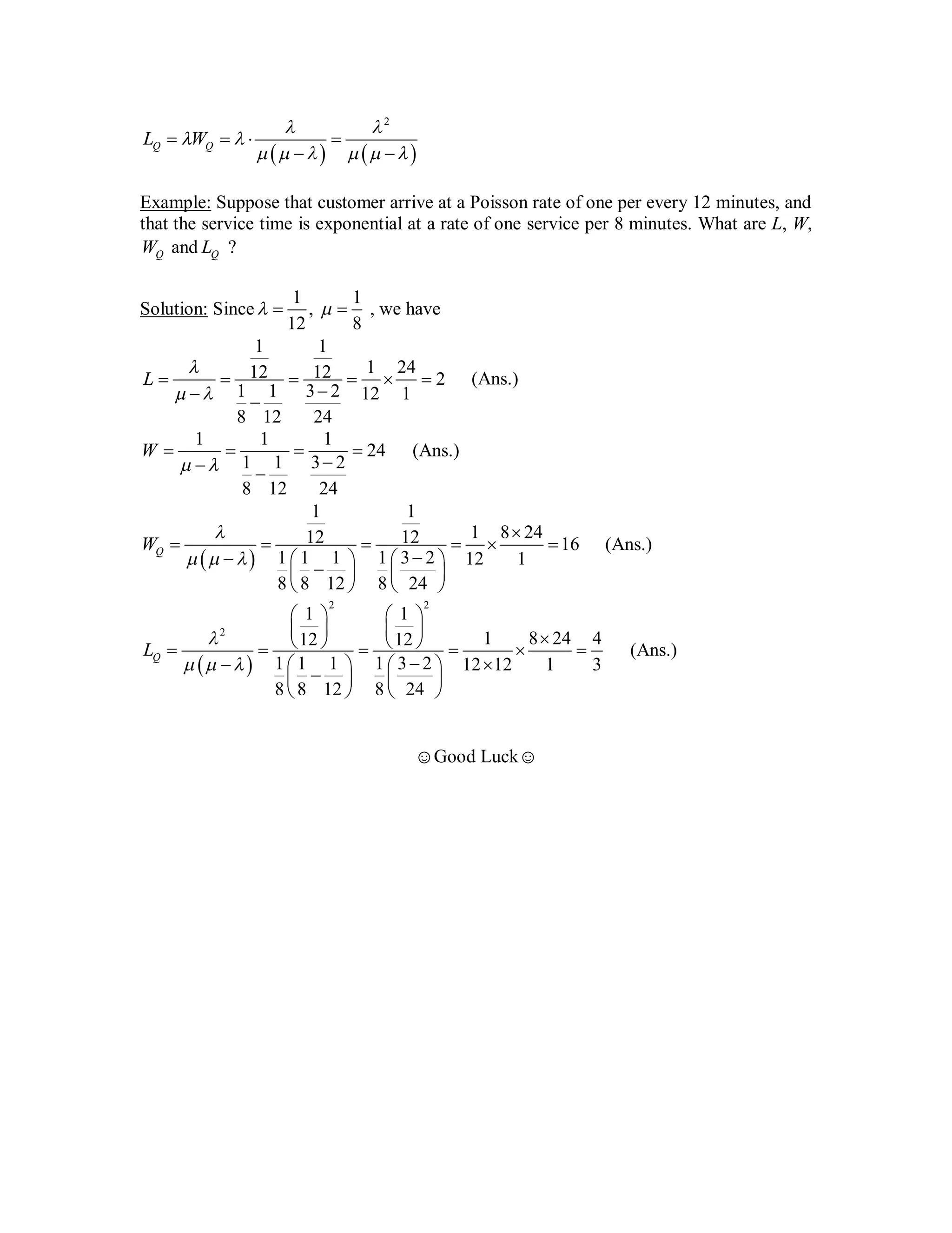
1
 
   
       
 
    
  

The quantities , andQ QW W L now can be obtained with the help of equations (1) and (2).
That is, since a  , we have from equation (5) that
  1 1L
W

  
      

    
 
   
1 1 1
[ ]QW W E S W
   
         
 
       
  
where, E[S] = average service time =
1

(for exponential distribution).
L = Average no. of customers in system
= Expected no. of customers in system
= E [customers in system]
= (sum over all possible n) n * Pn
L = (lambda) * W, Example: you waiting for 10 sec,
on average 5 customers/second ARRIVE
Then: no. of customers in the System will be 10 * 5 = 50
Thus, L = W * arrival rate (or, lambda) ==> W = L / lambda
(avg. service rate = MEU ... means
avg. service time = 1/MEU)

7.    
2
Q QL W
 
 
     
   
 
Example: Suppose that customer arrive at a Poisson rate of one per every 12 minutes, and
that the service time is exponential at a rate of one service per 8 minutes. What are L, W,
QW and QL ?
Solution: Since
1 1
,
12 8
   , we have
1 1
1 2412 12 2
1 1 3 2 12 1
8 12 24
L

 
     
 
(Ans.)
1 1 1
24
1 1 3 2
8 12 24
W
 
   
 
(Ans.)
 
1 1
1 8 2412 12 16
1 1 1 1 3 2 12 1
8 8 12 8 24
QW

  

     
    
   
   
(Ans.)
 
2 2
2
1 1
1 8 24 412 12
1 1 1 1 3 2 12 12 1 3
8 8 12 8 24
QL

  
   
            
    
   
   
(Ans.)
☺Good Luck☺
(Or, What is Average number of customers in the System? Average Waiting Time?
Average no. of Customers in Queue? And Waiting time in Queue?)
*Check: Meu must be > = lambda, otherwise infinity Queue
length and infinite waiting timw hobe !!! *
= 24 minutes
minutes
persons/minute
More Questions:
What is the probability that There are 5 customers in the System? (given: Lambda and Mu)
(Ans: Find P5, using the formula (4) for Pn from previous page. Just put n=5)
What is Probability that there will be at least 3 customers in the system?
Ans: P3 + P4 + P5 + ..... ... ... = 1 - P0 -P1 - P2 (find Pn from formula (4) for n=0,1,2)
What is Probability that the Single Server is IDLE in the system?
Ans: Server IDLE means no customers. The probability is P0 => put n=0 in formula (4)
to find out P0 = 1 - lambda/mu

8. Queuing Theory
A single-Server Exponential Queuing System Having Finite Capacity: In the previous model,
we assumed that there was no limit on the number of customers that could be in the system at
the same time. However, in reality there is always a finite system capacity N, in the sense that
there can be no more than N customers in the system at any time. By this, we mean that if an
arriving customer finds that there are already N customers present, then he does not enter the
system.
We let ,0nP n N  , denote the limiting probability that there are n customers in the system.
The rate-equality principle yields the following set of balance equations:
State Rate at which the process leaves = rate at which it enters
0 0 1P P 
1 1n N   1 1( ) n n nP P P      
N 1N NP P  
The equation for state 0 to N-1 is similar to single-server exponential queuing system with
infinite capacity. But, we have new equation for state N for finite capacity N. State N can only
be left via a departure since an arriving customer will not enter the system when it is in state N;
also state N can now only be entered from state 1N  via an arrival.
To solve, we again rewrite the preceding system of equations:
1 0
1 1
1
( ), 1 1n n n n
N N
P P
P P P P n N
P P


 
 


 


     

which, solving in terms of 0P , yields
Putting n = 0, we get 1 0P P



Putting n = 1, we get
2
2 1 1 0 1 0 0P P P P P P P
     
     
   
         
   
Putting n = 2, we get
2 3
3 2 2 1 2 0 0P P P P P P P
     
     
     
           
     

Putting n = N-1, we get
2 1
1 2 2 3 1 0 0
N N
N N N N NP P P P P P P
     
     
 
    
     
           
     
Putting n = N-1, we get
1
1 0 0
N N
N NP P P P
   
   


   
      
   
Single Server Exponential Queueing System with Finite Capacity OR
M/M/1Queue with Finite Queue or Buffer Length

9. By using the fact
0
1
N
n
n
P

 , we obtain
 
 
 
1
1
2
0 0
0 0
0 1
1
1
1 , 1
11
1
1
N
n nN n
i n
n i
N
x
P P x x x x
x
P










 

 
     
               
  

 

  
Hence,
 
 
   
 
0 1 1
1 1
, 0,1, ,
1 1
n
n n
n N N
P P n N
  
   
   
 
 
 
   
       
     

Now we can find out L putting the value of nP .
   
 
 
 
 
1
0 0
1
0
1
1
1
1
n
N N
n N
n n
nN
N
n
L nP n
n
 
 



 




 



 




 

We can solve  0
nN
n
n 

 using perturbation technique.
Though
1 2
2
0
( 1)
(1 )
n nn
k
k
x n x nx
kx
x
 

  


 (See Lec-5)
Similarly,  
    
 
1 2
2
0
1
1
N N
nN
n
N N
n
  
  



 

  



 
 
    
 
    
   
    
   
1 2
1 2
11 2
1 1
1 1
1 1
1 11
1 1
N N
N
N NN N
N N
N N
L
N NN N
   
   
 
 
       
   
  
 

 
 
   
 
 
 
      
  
    
      
    

10. In deriving W, the expected amount of time a customer spends in the system, we must be little
careful. If we have full capacity N customer in the system, then extra customers cannot enter
the system for service and they will not spend their time and money in the system. Thus we
should only consider those customers who get the chance to get service. Since the fraction of
arrivals that actually enter the system is1 NP , it follows that  1a NP   . Now, W can be
obtained from the following equation
    
       
 
    
         
 
    
       
1
1
1
1
1
1
1
1
1
1 1
1
1 1
1
1 1
1 1
1
1
1 1
1 1
N N
N
a
N
N
N N
N N
N
N
N N
N N
N N
L
W
N N
N N
 
 
  
   



 
 
  
   



 
 
   
  









 
   
  
 
  
    
   
  
 
   
 
 
    
    
   
  
 
   
 
 
    
 
We can also find out andQ QL W similarly like single-server exponential model with infinite
system.
Example: Suppose that it costs c dollars per hour to provide service at a rate  . Suppose
also that we incur a gross profit of A dollar for each customer served. If the system has a
capacity N, what service rate  maximizes our total profit?
Solution: Let, potential customers arrive at  rate. However, a certain proportion of them do
not join the system; namely, those who arrive when there are N customers already in the
system. Hence, since NP is the proportion of time that the system is full, it follows that
entering customer arrive at a rate of (1 )NP  . Since each customer pays $A, it follows that
money come in at an hourly rate of (1 )NP A  and since it goes out at an hourly rate ofc , it
follows that our hourly profit per hour is given by

11.    
 
     
 
 
 
1
1 1
1 1
profit per hour = (1 )
1
1
1
11
1 1
N
N
N
NN N N
N N
P A c
A c
A
A c c
 
 
 
 


     
  
 
 

 
 
 
 
 
   
 
  
              
  
  
For instance if 2, 1, 10, 1N A c    , then
 
 
   
2
2 33
3 2 3 3
110 1
10 1 10
profit per hour =
1 111
   
  
  

 
          
 

in order to maximize profit we differentiate to obtain
The value of that maximizes our profit now can be obtained by equating to zero and solving
numerically.
☺Good Luck☺
 
         
   
3 2 3 2
3 2 2
5 3 2 5 3 3 2
3 2 3 2
10 1 3 1 3
profit per hour 1,
( 1)
10 3 3 1 3 3 2 3 1
1 10 1
( 1) ( 1)
d d
v u u v
d d u dx dx
d dx v v
    
 
      
 
 
            
   
 
      
   
 


12. Queuing Theory
A Shoeshine Shop: Consider a shoeshine shop consisting of two chairs. Suppose that an
entering customer first will go to chair 1. When his work is completed in chair 1, he will go
either to chair 2 if that chair is empty or else wait in chair 1 until chair 2 becomes empty.
Suppose that a potential customer will enter this shop as long as chair 1 is empty. (Thus, for
instance, a potential customer might enter even if there is a customer in chair 2.)
If we suppose that potential customers arrive in accordance with a Poisson process at rate
and that the serving time for two chairs independent and have respective exponential
rates 1 2and  , then
(a) What proportion of potential customers enters the system?
(b) What is the mean number of customers in the system?
(c) What is the average amount of time that an entering customer spends in the system?
State Interpretation
(0,0) There are no customers in the system.
(1,0) There is one customer in the system and he is in chair 1.
(0,1) There is one customer in the system and he is in chair 2.
(1,1) There are two customers in the system and both are presently being served.
(b,1) There are two customers in the system but the customer in the first chair has completed
his work in that chair and is waiting for the second chair to become free.
It should be noted that when the system is in state (b,1), the person in chair 1, though not
being served is nevertheless “blocking” potential arrivals from entering the system. The
transition diagram given below shows all transition between above mentioned 5 states.
To write the balance equations we equate the sum of the arrows (multiplied by the probability
of the states where they originate) coming into a state with the sum of arrows (multiplied by
the probability of the state) going out of that state. This gives
 1, 0
 0,0
 0,1
 1,1
 ,1b
1

2
2
2
1
 
 
 
00 2 01
1 10 00 2 11
0,0
1,0
0,1
State Rate that the process leaves rate that it enters
P P
P P P
 
  


 
 
   
 
2 01 1 10 2 1
1 2 11 01
2 1 1 11
1,1
,1
b
b
P P P
P P
b P P
   
  
 
  
 

What proportion does not Enter?
What proportion of customers has to wait on
chair 1 after their service at chair 1 is over?
*** This is called the
State Transition Diagram
for the
Shoeshine Shop Model ***
Shoeshine Shop Model for the Queue

13. These along with the equation,
00 10 01 11 1 1bP P P P P    
may be solved to determine the limiting probabilities.
(a) Since a potential customer will enter the system when the state is either (0,0) or (0,1),
it follows that the proportion of customers entering the system is 00 01P P .
(b) Since there is one customer in the system whenever the state is (0,1) or (1,0) and two
customer in the system whenever the state is (1,1) or (b,1), it follows that L, the
average number of customer in the system is given by
 01 10 11 12 bL P P P P   
(c) To derive the average amount of time that an entering customer spends in the system,
we use the relationship
a
LW

 . Since a potential customer will enter the system
when in state (0,0) or (0,1), it follows that  00 01a P P   and hence
 
 
01 10 11 1
00 01
2 bP P P P
W
P P
  


Example: (a) If 1 21, 1, 2     , then calculate the preceding quantities of interest.
(b) If 1 21, 2, 1     , then calculate the preceding.
Solution: (a) Putting the values of 1 21, 1, 2     in probability equations, we get
00 01
10 00 11
01 10 1
11 01
1 11
2 (1)
2 (2)
3 2 (3)
3 (4)
2
b
b
P P
P P P
P P P
P P
P P

 
 






00 10 01 11 1
(5)
1 (6)bP P P P P    


From equation (6), we get
 00 00 11 00 11 11
00 01
00 00
00
00
1 1
2 1, [using equation (1), (2) and (5)]
2 2
5 7 1
=1, [using equation (4)]
2 2 3
5 7 1
1, [using equation (1)]
2 6 2
30 7
1
12
12
37
P P P P P P
P P
P P
P
P
     
  
   

 
 
Average (x) = E[x]
= x.Px
= 0*P00 + 1*P01 + 1*P10 + 2*P11 + 2*Pb1
W = L * lambda won't
work directly because
all of lambda (i.e., arrivals)
not effective (i.e.,
some ppl not entering)

14. Putting the value of 00P in equation (1), we get
01 01
12 6
2
37 37
P P  
Putting the value of 01P in equation (4), we get
11 11
6 2
3
37 37
P P  
Putting the value of 00 11andP P in equation (2), we get
10
12 2 16
2
37 37 37
P    
Putting the value of 11P in equation (5), we get
1 1
2 1
2
37 37
b bP P  
Hence, 00 01
12 6 18
37 37 37
P P    (Ans.)
 01 10 11 1
6 16 2 1 28
2 2
37 37 37 37 37
bL P P P P
 
         
 
(Ans.)
 
 
01 10 11 1
00 01
6 16 2 1
2
2 28 37 1437 37 37 37
12 6 37 18 9
37 37
bP P P P
W
P P
 
           
  
 
 
(Ans.)
Solution (b) is similar to (a). Try it yourself and check the answers are given below
00 01 11 10 1
3 3 1 2 2
, , , ,
11 11 11 11 11
bP P P P P    
Hence, 00 01
6 11
, 1,
11 6
P P L W   
*** There are many possible Questions for the exam, because Many Possible Quantities You
may have to find ! Following are some examples ...
The Probability (or, Fraction of Time) Both the Chairs are Empty (ans: find P00)
The Probabilty that Chair 1 is empty (find P00+P01)
The Fraction of Time Chair 2 is empty (ans: find P00 + P10)
The Probability Chair 2 is Filled (ans: find P01 + P11 + Pb1)
The fraction of time Either or Both Chairs Filled = (1 - P00) OR (P01+P10+P11+Pb1)
The Probabilty that Both the chairs are filled = P11 + Pb1