Control system

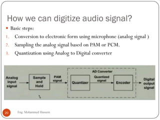
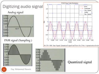
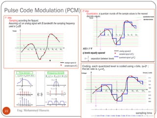
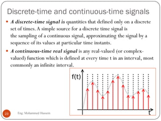
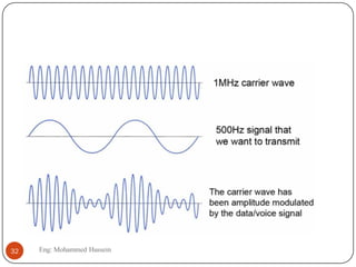
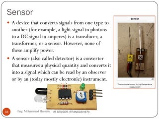
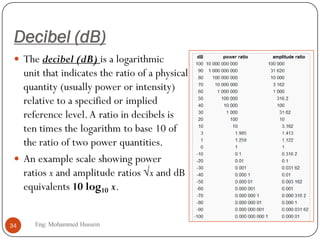
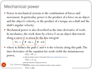
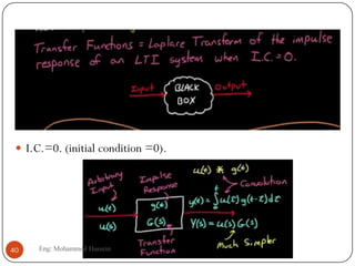
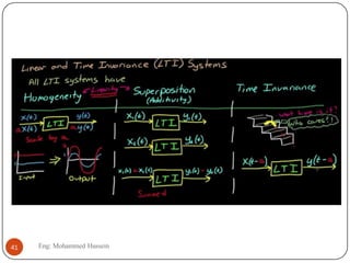
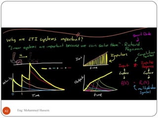
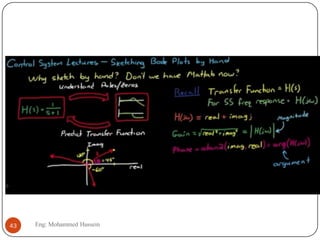
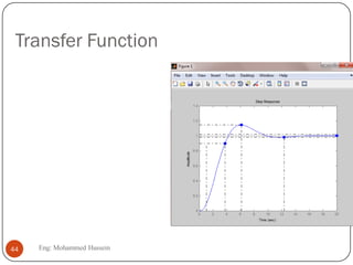
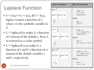
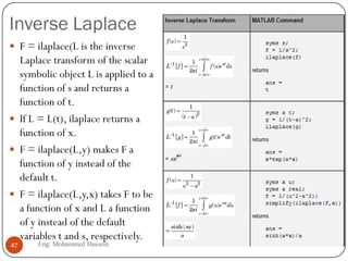
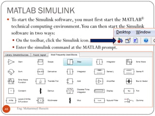
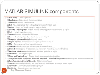
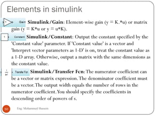
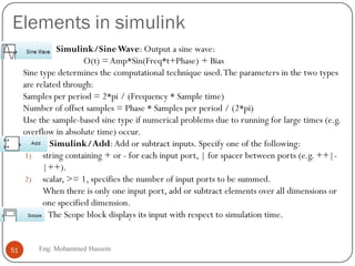
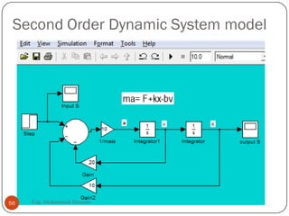
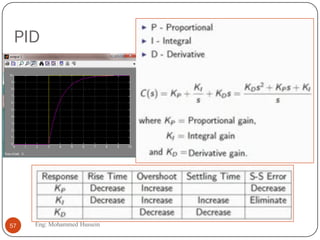
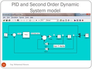
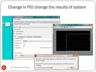
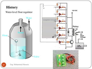
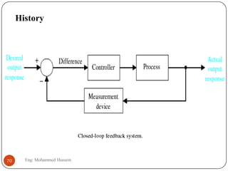
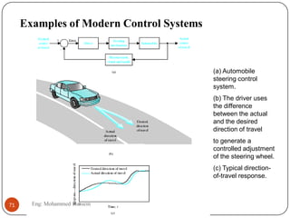
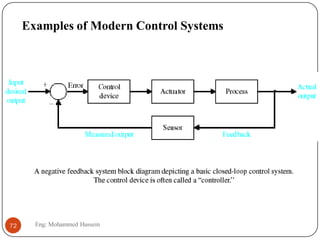
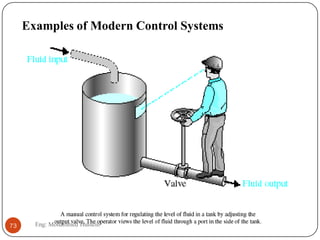
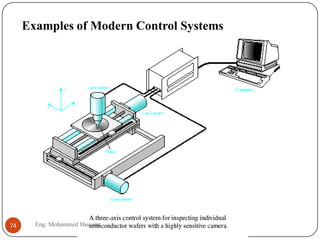
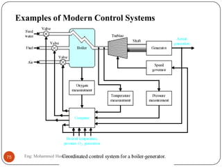
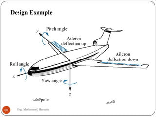
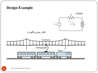
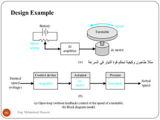
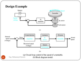
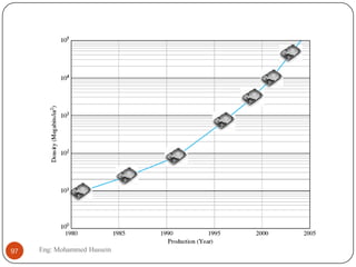
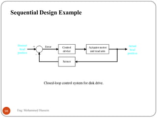
Eng: Mohammed Hussein1
Republic of Yemen
THAMAR UNIVERSITY
Faculty of Computer Science&
Information System
Lecturer, and Researcher atThamar University
By Eng: Mohammed Hussein

History
18th Century James Watt’s centrifugal governor for the speed control of a steam
engine.
1920s Minorsky worked on automatic controllers for steering ships.
1930s Nyquist developed a method for analyzing the stability of controlled systems
1940s Frequency response methods made it possible to design linear closed-loop
control systems
1950s Root-locus method due to Evans was fully developed
1960s State space methods, optimal control, adaptive control and
1980s Learning controls are begun to investigated and developed.
Present and on-going research fields. Recent application of modern control theory
includes such non-engineering systems such as biological, biomedical, economic and
socio-economic systems
???????????????????????????????????
2 Eng: Mohammed Hussein

Introduction to Control Systems
Objectives
 We will describe a general process for designing a control system.
 A control system consisting of interconnected components is designed to
achieve a desired purpose.
 To understand the purpose of a control system, it is useful to examine
examples of control systems through the course of history. These early
systems incorporated many of the same ideas of feedback that are in use
today.
 Modern control engineering practice includes the use of control design
strategies for improving manufacturing processes, the efficiency of energy
use, advanced automobile control, including rapid transit, among others.
 The iterative nature of design allows us to handle the design gap effectively
while accomplishing necessary tradeoffs in complexity, performance, and cost
in order to meet the design specifications.

Introduction
 A study of control involves developing a mathematical model for each
component of the control system.
 A system is a set of self-contained processes under study.
 A control system by definition consists of the system to be controlled -
called the plant - as well as the system which exercises control over the
plant, called the controller.A controller could be either human, or an
artificial device.The controller is said to supply a signal to the plant, called
the input to the plant (or the control input), in order to produce a desired
response from the plant, called the output from the plant.When referring
to an isolated system, the terms input and output are used to describe the
signal that goes into a system, and the signal that comes out of a system,
respectively.

Example of control system
 If we select the car to be the plant, then the driver becomes the
controller, who applies an input to the plant in the form of pressing
the gas pedal if it is desired to increase the speed of the car.The
speed increase can then be the output from the plant.

Introduction
System – An interconnection of elements and devices for a desired purpose.
Control System – An interconnection of components forming a system
configuration that will provide a desired response.
Process – The device, plant, or system
under control. The input and output
relationship represents the cause-and-
effect relationship of the process.

Introduction
Multivariable Control System
Open-Loop Control Systems
utilize a controller or control
actuator to obtain the desired
response.
Closed-Loop Control
Systems utilizes feedback to
compare the actual output to
the desired output response.

Plan of study
 Information, picture and video for system
 Math
 Apply in Matlab
 Using simulink and output of system
 Response of the human ear (20 Hz to 20 KHz, sensitive to changes
to signal levels rather than absolute values, for animal can be more
then human ).

A Simple Feedback Control Example

Hardware elements
 Series R
 Model series resistor
 Series C
 Model series capacitor
 Series L
 Model series inductor
 Library
 Ladders Filters sublibrary of the Physical library
 Description
The Series R,C,L blocks models described in the block
dialog box, in terms of its frequency-dependent S-parameters.

Series RLC
 Series RLC Branch
 Implement series RLC branch
 Library
 Elements
 Description
The Series RLC Branch block implements a single resistor,
inductor, or capacitor, or a series combination of these. Use the
Branch type parameter to select elements you want to include
in the branch.

Signal
 A signal is a function that conveys information about the behavior
or attributes of some phenomenon.
 The IEEETransactions on Signal Processing definition as:
 The term "signal" includes, among others, audio, video,
speech, image, communication, geophysical, sonar, radar, medical and
musical signals.
 There are types of signal such as:
1. Discrete-time and continuous-time signals
2. Analog and digital signals

Pulse Step Signal

Pulse Step

Types of Waveforms (periodic) Signals

Waveforms (Aperiodic) Signal

Types of Waveforms (Aperiodic) Signals

Why we use these signals?
 Based on these Signals we can create complex Signals.
 Sinusoid, unit step and exponential are used to approximate
basically more complex signals.
 They help us to predict and analysis as we take the signals as input
to the system such as filters, high pass, low pass, band pass, etc
filters and see what the output is.

How we can digitize audio signal?
 Basic steps:
1. Conversion to electronic form using microphone (analog signal )
2. Sampling the analog signal based on PAM or PCM.
3. Quantization using Analog to Digital converter

Digitizing audio signal
Analog signal
PAM signal (Sampling )
Quantized signal

Pulse Code Modulation (PCM)

Discrete-time and continuous-time signals
 A discrete-time signal is quantities that defined only on a discrete
set of times.A simple source for a discrete time signal is
the sampling of a continuous signal, approximating the signal by a
sequence of its values at particular time instants.
 A continuous-time real signal is any real-valued (or complex-
valued) function which is defined at every time t in an interval, most
commonly an infinite interval.

Analog and digital signals
 The figure shows a digital signal that results from approximating
an analog signal by its values at particular time instants. Digital
signals are discrete and quantized, while analog signals possess
neither property.

Direct current (DC)
 Direct current (DC) is the unidirectional flow of electric charge. Direct
current is produced by sources such as batteries, thermocouples, solar
cells, and commutator-type electric machines of the dynamo type.
 The electric charge flows in a constant direction, distinguishing it
from Alternating current (AC). A term formerly used for direct
current was galvanic current.The abbreviationsAC and DC are often used
to mean simply alternating and direct, as when they
modify current or voltage.
Direct Current (red curve). The horizontal axis
measures time; the vertical, current or voltage.
Types of direct current.

DC signals
 It does not change over time.

Voltage or Current over time

Amplitude modulation

Amplifier
 An amplifier is a device for increasing the power of a signal by use of an
external energy source.
 In an electronic amplifier, the input "signal" is usually a voltage or a
current.
 Amplifiers may be classified in a variety of ways depending on their
application, the frequency range they cover, or the active devices used.
Ideally an amplifier increases the power of a signal without otherwise
altering it; practical amplifiers have finite distortion and noise which they
invariably add to the signal.
 DC integrated amplifier
 DC(Direct Coupled) using no capacitors in the audio path.
 Integrated = Power amplifier and Pre-amplifier 'integrated' together in one
box.

Sensor
 A device that converts signals from one type to
another (for example, a light signal in photons
to a DC signal in amperes) is a transducer, a
transformer, or a sensor. However, none of
these amplify power.
 A sensor (also called detector) is a converter
that measures a physical quantity and converts it
into a signal which can be read by an observer
or by an (today mostly electronic) instrument.

Decibel (dB)
 The decibel (dB) is a logarithmic
unit that indicates the ratio of a physical
quantity (usually power or intensity)
relative to a specified or implied
reference level.A ratio in decibels is
ten times the logarithm to base 10 of
the ratio of two power quantities.
 An example scale showing power
ratios x and amplitude ratios √x and dB
equivalents 10 log10 x.

Mechanical power
 Power in mechanical systems is the combination of forces and
movement. In particular, power is the product of a force on an object
and the object's velocity, or the product of a torque on a shaft and the
shaft's angular velocity.
 Mechanical power is also described as the time derivative of work.
In mechanics, the work done by a force F on an object that travels
along a curve C is given by the line integral:
 where x defines the path C and v is the velocity along this path.The
time derivative of the equation for work yields the instantaneous
power,

Electrical power
 The instantaneous electrical power P delivered to a component is
given by: where:
 P(t) is the instantaneous power, measured
in watts (joules per second).
 V(t) is the potential difference (or voltage drop) across the
component, measured in volts.
 I(t) is the current through it, measured in amperes
 If the component is a resistor with time-
invariant voltage to current ratio, then:

Mechanical advantage
The law of the lever
 The lever is a movable bar that pivots on a fulcrum attached to or
positioned on or across a fixed point.The lever operates by applying
forces at different distances from the fulcrum, or pivot.
 As the lever pivots on the fulcrum, points farther from this pivot move
faster than points closer to the pivot.The power into and out of the
lever must be the same, so forces applied to points farther from the
pivot must be less than when applied to points closer in.
 If a and b are distances from the fulcrum to pointsA and B and if
force FA applied toA is the input force and FB exerted at B is the
output, the ratio of the velocities of pointsA and B is given by a/b, so
the ratio of the output force to the input force, or mechanical
advantage, is given by

Mechanical advantage- Speed ratio
 The requirement for power input to an ideal mechanism to equal power
output provides a simple way to compute mechanical advantage from
the input-output speed ratio of the system.
 Power is the product of force and velocity.The power input to a gear
train with a torqueTA applied to the drive pulley which rotates at an
angular velocity of ωA is P=TA ωA.
 Because the power flow is constant, the torque TB and angular
velocity ωB of the output gear must satisfy the relation
 This shows that for an ideal mechanism the input-output speed ratio
equals the mechanical advantage of the system.

Complex Numbers
 Where σ is the real part and ῳ is the imaginary part. The basic imaginary unit is equal to
the square root of -1.This is represented in MATLAB by either of two letters: i or j.
 The variable x is assigned a complex number with a real part of 2 and an imaginary part of
3.
 Another way to create a complex number is using the complex function.
 A complex function G(s),a function of s,has a real part and an imaginary part
 This function combines two numeric inputs into a complex output, making the first input
real and the second imaginary.
 You can separate a complex number into its real and imaginary parts using the real and
imag functions.
x = 2 + 3i;
x = rand(3) * 5;
y = rand(3) * -8;
z = complex(x, y);
zr = real(z);
zi = imag(z);

 I.C.=0. (initial condition =0).

Transfer Function

Laplace transform method
 The Laplace transform method is an operational method that can be used
advantageously for solving linear differential equations. By use of Laplace transforms,
we can convert many common functions, such as sinusoidal functions, damped
sinusoidal functions, and exponential functions, into algebraic functions of a complex
variable s. Operations such as differentiation and integration can be replaced by
algebraic operations in the complex plane.Thus, a linear differential equation can be
transformed into an algebraic equation in a complex variable s. If the algebraic
equation in s is solved for the dependent variable, then the solution of the differential
equation (the inverse Laplace transform of the dependent variable) may be found by
use of a Laplace transform table or by use of the partial-fraction expansion technique.
 An advantage of the Laplace transform method is that it allows the use of graphical
techniques for predicting the system performance without actually solving system
differential equations.Another advantage of the Laplace transform method is that,
when we solve the differential equation, both the transient component and steady-
state component of the solution can be obtained simultaneously.

Laplace Function
 F = F(s)=>L = L(t), If F = F(s),
laplace returns a function of t.
where t is the symbolic variable in
F.
 L = laplace(F,t) makes L a function
of t instead of the default s. Here L
is returned as a scalar symbol.
 L = laplace(F,w,z) makes L a
function of z and F a function of w
instead of the default variables s
and t, respectively.

Inverse Laplace
 F = ilaplace(L is the inverse
Laplace transform of the scalar
symbolic object L is applied to a
function of s and returns a
function of t.
 If L = L(t), ilaplace returns a
function of x.
 F = ilaplace(L,y) makes F a
function of y instead of the
default t.
 F = ilaplace(L,y,x) takes F to be
a function of x and L a function
of y instead of the default
variables t and s, respectively.

MATLAB SIMULINK
 To start the Simulink software, you must first start the MATLAB®
technical computing environment.You can then start the Simulink
software in two ways:
 On the toolbar, click the Simulink icon.
 Enter the simulink command at the MATLAB prompt.

MATLAB SIMULINK components

Elements in simulink
 Simulink/Gain: Element-wise gain (y = K.*u) or matrix
gain (y = K*u or y = u*K).
 Simulink/Constant: Output the constant specified by the
'Constant value' parameter. If 'Constant value' is a vector and
'Interpret vector parameters as 1-D' is on, treat the constant value as
a 1-D array. Otherwise, output a matrix with the same dimensions as
the constant value.
 Simulink/Transfer Fcn:The numerator coefficient can
be a vector or matrix expression.The denominator coefficient must
be a vector.The output width equals the number of rows in the
numerator coefficient.You should specify the coefficients in
descending order of powers of s.

Elements in simulink
 Simulink/SineWave: Output a sine wave:
O(t) = Amp*Sin(Freq*t+Phase) + Bias
Sine type determines the computational technique used.The parameters in the two types
are related through:
Samples per period = 2*pi / (Frequency * Sample time)
Number of offset samples = Phase * Samples per period / (2*pi)
Use the sample-based sine type if numerical problems due to running for large times (e.g.
overflow in absolute time) occur.
 Simulink/Add:Add or subtract inputs. Specify one of the following:
1) string containing + or - for each input port, | for spacer between ports (e.g. ++|-
|++).
2) scalar, >= 1, specifies the number of input ports to be summed.
When there is only one input port, add or subtract elements over all dimensions or
one specified dimension.
 The Scope block displays its input with respect to simulation time.

Getting Started with Simulink
‫الوعالج‬ ‫حرارة‬ ‫لقياس‬ ‫نظام‬

First Order Dynamic System
 The Mass block represents an ideal mechanical translational mass

First Order Dynamic System model

Second Order Dynamic System

Second Order Dynamic System model

PID and Second Order Dynamic
System model

Change in PID change the results of system

Auto control: Response time
&Parameters

Open-loop bode plot of the system

System Results and error

 K=1
 Here is the Imaginary Axis.
 when you have your system
result poles after theAxis,
you would have unstable
system.
 Also Step Response is stable
Step Response is stable

Changing K controller value
 When we change k=6 which is near to Imaginary Axis, we have
unstable system that represented in Step Response figure.

History
Water-level float regulator

ESP-SMT Smart Control System

Traction Control System

History

(a) Automobile
steering control
system.
(b) The driver uses
the difference
between the actual
and the desired
direction of travel
to generate a
controlled adjustment
of the steering wheel.
(c) Typical direction-
of-travel response.
Examples of Modern Control Systems

A Robot Balanced on a Ball
Tohoru gakuin university
Robot development engineering lab79 Eng: Mohammed Hussein

The Future of Control Systems

Control System Design

Design Example

Steam-driven Electric Power Plant
1. Cooling tower
2. Cooling water pump or Circulating water pump
3.Transmission line (3-phase)
4. Step-up transformer (3-phase)
5. Electric generator (3-phase)
6. Low pressure turbine
7a. Condensate pump
7b. Boiler Feedwater pump
8. Condenser
9. Intermediate pressure turbine
10. Steam governor or control valve
11. High pressure turbine
12. Deaerator
13. Feed heater
14. Reheater section (if any)
15. Steam generating heat source
16. Moisture separators

ELECTRIC SHIP CONCEPT
Ship
Service
Power
Main Power
Distribution
Propulsion
Motor
Motor
Drive
Generator
Prime
Mover
Power
Conversion
Module
 Electric Drive
 Reduce # of Prime
Movers
 Fuel savings
 Reduced maintenance
 Technology
Insertion
 Warfighting
Capabilities
Vision
Integrated
Power
System
All
Electric
Ship
Electrically
Reconfigurable
Ship
 Reduced manning
 Automation
 Eliminate auxiliary
systems (steam,
hydraulics, compressed
air)
IncreasingAffordability and Military Capability
Design Example

CVN(X) FUTURE AIRCRAFT CARRIER
Design Example
‫الطائرات‬ ‫حاهلة‬

Design Example
‫التدوير‬
‫القطب‬pole

Design Example
‫بالكهرباء‬ ‫يوشي‬ ‫قطار‬
‫العجالت‬

Design Example
‫السرعة‬ ‫في‬ ‫التيار‬ ‫قىة‬ ‫تحكن‬ ‫وكيفية‬ ‫طاحىى‬ ‫هثال‬

Design Example

Sequential Design Example

References, and Resources
 http://en.wikipedia.org/wiki/Signal_(information_theory)
 http://en.wikipedia.org/wiki/Electronic_amplifier.
 http://en.wikipedia.org/wiki/Amplifier.
 http://en.wikipedia.org/wiki/Decibel

Control system

More Related Content

What's hot

Viewers also liked

Similar to Control system

More from Mohammed Hussein

Recently uploaded

Control system