The document discusses the concept of limits in calculus. It defines a limit and provides examples to build intuition. Some key points made in the document include: 1) A limit describes the behavior of a function as the input values get closer to a specific value without actually reaching it. 2) Basic theorems for limits include properties like the limit of a sum being the sum of the limits. 3) Special cases like limits with zero in the denominator require factoring to find the limit. 4) One-sided or directional limits describe the behavior of a function as the input approaches a value from the left or right.

1. 1
LIMITS
The fundamental idea of the calculus is the concept of limit. The exercises in Part I
are designed to improve your understanding and skills in working with this con-
cept. The symbolisms involved are useful contractions/abbreviations and recogniz-
ing the “form” of these is essential in successfully producing required results. Before
you begin, if you need a review of functions, see Appendix A: Basic functions and
their graphs.
·I·

2. This page intentionally left blank

3. 3
Limit definition and intuition
A function f x( ) is said to have a limit A as x approaches c written lim ( )
x c
f x A,
provided the error between f x( ) and A, written | ( ) |f x A , can be made less than
any preassigned positive number whenever x is close to, but not equal to, c. Heu-
ristically, “The limit of f at the point c is A if the value of f gets near A when x is near c.”
We will explore this definition intuitively through the following examples.
Compute the value of f x x( ) 2
5 for the following values of x that are close
to, but not equal to 2 in value; and then make an observation about the
results.
a. x 2.07 f x( ) 9.2849
b. x 1.98 f x( ) 8.9204
c. x 2.0006 f x( ) 9.00240036
Observation: It appears that when x is close to 2 in value, then f(x) is close to
9 in value.
Compute the value of f x
x
( )
4
for the following values of x that are close to,
but not equal to 0 in value, and then make an intuitive observation about the
results.
a. x .01 f x( ) 400
b. x –.001 f x( ) –4000
c. x .001 f x( ) 4000
Observation: It appears that when x is close to 0 in value, f(x) is not close to
any fixed number in value.
Using limit notation, you can represent your observation statements for the
above examples, respectively, as:
lim
x
x
2
2
5 9 and lim
x x0
4
does not exist.
The limit concept ·1·

4. 4 Limits
1·1
EXERCISE
Compute the value of f(x) when x has the indicated values given in (a) and (b). For (c), make
an observation based on your results in (a) and (b).
1. f x( )
x
x
2
5
a. x 3.001
b. x 2.99
c. Observation? ________________________________________________________
2. f x( )
x
x
5
4
a. x 1.002
b. x .993
c. Observation? ________________________________________________________
3. f x( )
3 2
x
x
a. x .001
b. x .001
c. Observation? ________________________________________________________
Properties of limits
Basic theorems that are designed to facilitate work with limits exist, and these theorems are the
“bare bones” ideas you must master to successfully deal with the limit concept. Succinctly, the
most useful of these theorems are the following:
If lim ( )
x c
f x and lim ( )
x c
g x both exist, then
1. The limit of the sum (or difference) is the sum (or difference) of the limits.
lim[ ( ) ( )]
x c
f x g x lim ( ) lim ( )
x c x c
f x g x
2. The limit of the product is the product of the limits.
lim[ ( ) ( )]
x c
f x g x lim ( ) lim ( )
x c x c
f x g x
3. The limit of a quotient is the quotient of the limits provided the denominator limit is not 0.
lim
( )
( )x c
f x
g x
lim ( )
lim ( )
x c
x c
f x
g x
4. If f x f x f x
x c
n
x c
n( ) 0, then lim ( ) lim ( )for n 0
5. lim ( ) lim ( )
x c x c
af x a f x where a is a constant
6. lim[ ( )] lim ( )
x c x c
n
f x f x
n
for any positive integer n
7. lim
x c
x c
8. lim
x c x c
1 1
provided c 0

5. The limit concept 5
You must guard against the error of writing or thinking that lim ( )
x c
f x f c( ); that is, that you
determine the limit by substituting x c into the expression that defines f(x) and then evaluate.
Recall that in the limit concept, x cannot assume the value of c. The complete explanation re-
quires the concept of continuity, which is discussed in Chapter 3.
PROBLEMS Evaluate the following limits.
a. lim
x
x
x2
3 5
5 2
b. lim( )
x
x x
4
3 16
c. lim
x
x
x4
2
16
4
SOLUTIONS a. lim
lim
limx
x
x
x
x
x
x2
2
2
3 5
5 2
3 5
5 2
1
12
b. lim( ) lim lim lim
x x x x
x x x x x
4 4 4 4
3 16 3 16 3 llim16 12 64 20
4
x
x
c. lim lim
( )( )
lim(
x x x
x
x
x x
x
x
4
2
4 4
16
4
4 4
4
4 8)
Notice that in this example, you cannot use the quotient theorem because the limit of the
denominator is zero; that is, lim( )
x
x
4
4 0. However, as shown, you can take an algebraic ap-
proach to determine the limit. First, you factor the numerator. Next, using the fact that for all
x
x x
x
x4
4 4
4
4,
( )( )
, you can simplify the fraction and then evaluate the limit. This is a
useful approach that can be applied to a number of limit problems.
d. lim
x
x
1
6 12 does not exist because 6x 12 0 when x is close to 1.
1·2
EXERCISE
Find the following limits or indicate nonexistence.
1. lim
x
x
x3
2
4
1
6. lim
x
x
x0
2
3
9 3
11
2. lim
x
x
x2
2
9
2
7. lim
x
x x
x1
2
2
2 1
1
3. lim
x
x
1
3
7 8. lim
x
x
x4 2
6 3
16
4. lim( )
x
x5 92
9. lim
x
x
2
3
4 11
5. lim
x
x
x0
5 3
11
10. lim
x
x
x6
8 3
6

6. This page intentionally left blank

7. 7
Zero denominator limits
Some of the most useful limits are those in which the denominator limit is 0, even
though our previous limit theorems are not directly applicable in these cases.
These types of limits can exist only if there is some sort of cancellation com-
ing from the numerator. The key is to seek common factors of the numerator and
denominator that will cancel.
PROBLEMS Evaluate the following limits.
a. lim
x
x
x4
3
8
2
b. lim
( ) ( )
h
x xh h x
h0
2 2 2
5 10 5 2 5 2
c. lim
h
x h x
h0
SOLUTIONS a. lim lim
( )( )
lim
x x x
x
x
x x x
x4
3
4
2
8
2
2 2 4
2 44
2
2 4 28( )x x
b. lim
( ) ( )
lim
h h
x xh h x
h
xh
0
2 2 2
0
5 10 5 2 5 2 10 55 2
h
h
lim( )
h
x h x
0
10 5 10
c. lim lim
( )( )
( )h h
x h x
h
x h x x h x
h x h x0 0
lim
( )
( )
lim
( )h h
x h x
h x h x
h
h x h x0 0
lim
( )h
x h x x0
1 1
2
PROBLEM If f(x) 6x2 7, then find lim
( ) ( )
h
f x h f x
h0
.
SOLUTION lim
( ) ( )
lim
( ( ) ) (
h h
f x h f x
h
x h x
0 0
2 2
6 7 6 7))
h
lim
h
x xh h x
h0
2 2 2
6 12 6 7 6 7
lim( )
h
x h x
0
12 6 12
Special limits ·2·

8. 8 Limits
2·1
EXERCISE
Evaluate the following limits.
1. lim
x
x
x x3 2
3
12
2. lim
( )
h
x h x
h0
2 2
3. lim
x
x
x4
3
2
64
16
4. If f x x( ) 5 8, find lim
( ) ( )
h
f x h f x
h0
.
5. lim
x
x
x3 2
5 7
3
6. lim
x
x
x25
5
25
7. If g x x( ) 2
, find lim
( ) ( )
x
g x g
x2
2
2
.
8. lim
x
x x
x0
2
2 4
9. lim
r
x r x
r0
10. lim
x
x
x4
3
6
4
Infinite limits and limits involving infinity
The variable x is said to approach ( )if x increases (decreases) without bound. For example, x
approaches if x assumes the values 2, 3, 4, 5, 6, and so on, consecutively. Note, however, that y
does not approach infinity if y assumes the values 2, –2, 4, –4, 6, –6, and so on, in the same
manner.
A function becomes positively infinite as x approaches c if for every M 0, f(x) M for
every x close to, but not equal to, c. Similarly, a function becomes negatively infinite as x ap-
proaches c if for every M 0, f(x) M for every x close to, but not equal to, c.
PROBLEMS Evaluate the following limits.
a. lim ,
x
a
x
where a is any constant
b. lim
x
x2
c. lim
x
x
x
3 12
1
d. lim
| |x x3
4
3

9. Special limits 9
SOLUTIONS a. lim
x
a
x
0 for any constant a
b. lim
x
x2
c. lim lim
x x
x
x
x
x
3 12
1
3
12
1
1
3 0
1 0
3
d. lim
| |x x3
4
3
2·2
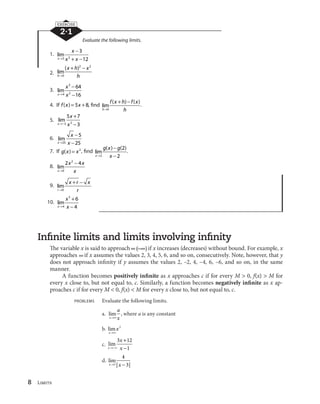
EXERCISE
Evaluate the following limits.
1. lim( )
x
x5 7 6. lim
x
x
x x
2
5 62
2. lim
x x
7
3
7. lim
x
x x
x x
5 3
6 2
6 7
5 6 11
3. lim
x
x3 95 8. lim
x
x x x
x x
7 6 3
3 7 5
4 2
3
4. lim
x
x x x
x x
3 2
3
47 9
18 76 11
9. lim
x
x x
x
2 8 5
3 4
3
2
5. lim
x x
8
4
10. lim
x x
5
42
Left-hand and right-hand limits
Directional limits are necessary in many applications and we write lim ( )
x c
f x to denote the limit
concept as x approaches c through values of x larger than c. This limit is called the right-hand
limit of f at c; and, similarly, lim ( )
x c
f x is the notation for the left-hand limit of f at c.
Theorem: lim ( )
x c
f x L if and only if lim ( ) lim ( )
x c x c
f x f x L. This theorem is a very useful tool
in evaluating certain limits and in determining whether a limit exists.
PROBLEMS Evaluate the following limits.
a. lim
x x3
4
3
b. lim
x x1
15
1
c. lim[ ]
x
x
2
Note: [x] denotes the greatest integer function (See Appendix A)

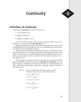
10. 10 Limits
d. lim[ ]
x
x
2
e. lim[ ]
x
x
2
SOLUTIONS a. lim
x x3
4
3
b. lim
x x1
15
1
c. lim[ ]
x
x
2
2
d. lim[ ]
x
x
2
1
e. lim[ ]
x
x
2
does not exist because lim[ ]
x
x
2
2 and lim[ ]
x
x
2
1, so the right- and
left-hand limits are not equal.
2·3
EXERCISE
Evaluate the following limits if they exist. If a limit does not exist, show why.
1. lim[ ]
x
x
4
1 6. lim
x
x
x3
2
9
3
2. lim
x
x
x2
2
4
2
7. lim
x x4
7
4
3. lim
x x8
4
9
8. lim
x
x x
x4
5 4
8
4
4. lim
x
x
0
4 3 9. lim
x
x
x4
2
16
4
5. lim[ ]
x
x
5
1 10. lim
x
x
x4
2
16
4

11. 11
Continuity
Definition of continuity
A function f is continuous at a point c if and only if
1. f c( )is defined; and
2. lim ( ) ;
x c
f x exists and
3. lim ( ) (lim ) ( ).
x c x c
f x f x f c
If a function fails to satisfy any one of these conditions, then it is not con-
tinuous at x c and is said to be discontinuous at x c.
Roughly speaking, a function is continuous if its graph can be drawn with-
out lifting the pencil. Strictly speaking, this is not mathematically accurate, but it
is an intuitive way of visualizing continuity.
Notice that when a function is continuous at a point c, you have the situation
whereby the limit may be calculated by actually evaluating the function at the
point c. Recall that you were cautioned against determining limits this way in an
earlier discussion; however, when a function is known to be continuous at x c,
then lim ( ) ( ).
x c
f x f c
By its definition, continuity is a point-wise property of a function, but this
idea is extended by saying that a function is continuous on an interval a x b
if and only if f is continuous at each point in the interval. At the end points, the
right- and left-hand limits apply, respectively, to get right and left continuity if
these limits exist.
PROBLEMS Determine whether the following functions are either
continuous or discontinuous at the indicated point.
a. f x x( ) 4 7 at x 4
b. f x x( ) 4 at x 3
c. f x x( ) 3 72
at x 2
d. f x
x
( )
12
2
at x 2
e. f x
x
x
( )
2
4
2
at x 2
·3·

12. 12 Limits
SOLUTIONS a. lim lim( ) (lim ) ;
x x x
x x x
4 4 4
4 7 4 7 4 7 23 thus, the
function is continuous at 4.
b. lim( ) ((lim ) ) ;
x x
x x
3 3
4 4 1 thus, the function is continuous at 3.
c. lim( ) ( (lim ) ) ;
x x
x x
2
2
2
2
3 7 3 7 19 thus, the function is continuous at 2.
d. lim
x x2
12
2
does not exist; thus, the function is discontinuous at 2.
e. f x
x
x
( )
2
4
2
is discontinuous at 2 because the function is not defined at 2.
However, the limit of f(x) as x approaches 2 is 4, so the limit exists but
lim ( ) ( ).
x
f x f
2
2 If f ( )2 is now defined to be 4 then the “new” function f(x)
x
x
x
x
2
4
2
2
4 2
is continuous at 2. Since the discontinuity at 2 can be “removed,”
then the original function is said to have a removable discontinuity at 2.
3·1
EXERCISE
Show that the following functions are either continuous or discontinuous at the indicated
point.
1. f x x( ) 5 7 at x 1 6. g x
x
x
( )
5
5
at x 3
2. f x
x
x
( )
3
8
2
at x 0 7. g x
x
x
( )
5
2
at x 8
3. f x
x
( )
4
2 3
at x 1 8. h x x x( ) 5 72
at x 5
4. f x x( ) [ ] at x 3 9. f x
x
x
( )
6
2
at x 6
5. g x
x
x
( )
2
6
5
at x 4 10. h x
x a x
x a
( )
( )2
6
3
at x a
Properties of continuity
The arithmetic properties of continuity follow immediately from the limit properties in Chapter 1.
If f and g are continuous at x c, then the following functions are also continuous at c:
1. Sum and difference: f g
2. Product: fg
3. Scalar multiple: af, for a a real number
4. Quotient:
f
g , provided g c( ) 0

13. Continuity 13
Further, if g is continuous at c and f is continuous at g(c) then the composite function f g
defined by ( )( ) ( ( ))f g x f g x is continuous at c. In limit notation, lim ( ( )) (lim ( ))
x c x c
f g x f g x
f g c( ( )). This function composition property is one of the most important results of continuity.
If a function is continuous on the entire real line, the function is everywhere continuous;
that is to say, its graph has no holes, jumps, or gaps in it. The following types of functions are
continuous at every point in their domains:
Constant functions: f(x) k, where k is a constant
Power functions: f x xn
( ) , where n is a positive integer
Polynomial functions: f x a x a x a x an
n
n
n
( ) 1
1
1 0
Rational functions: f x
p x
q x
( )
( )
( )
, provided p x( ) and q x( ) are polynomials and q x( ) 0
Radical functions: f x x xn
( ) , ,0 n a positive integer
Trigonometric functions: f(x) sinx and f(x) cosx are everywhere continuous; f(x) tan x,
f(x) cscx, f(x) secx, and f(x) cotx are continuous only wherever they exist.
Logarithm functions: f x x( ) ln and f x x b bb
( ) log , ,0 1
Exponential functions: f x ex
( ) and f x b b bx
( ) , ,0 1
PROBLEM Discuss the continuity of the following function: g x x( ) (sin )3 3 at a real number c.
SOLUTION 3x is continuous at c and sinx is continuous at all real numbers and so sin( )3x is
continuous at c by the composition property. Finally, 3 3sin( )x is continuous at c
by the constant multiple property of continuity.
3·2
EXERCISE
Discuss the continuity of the following functional expressions.
1. f x x( ) (tan )5 3 at a real number c 6. G x
x x
x
( )
sin
11 8 92
on the real line
2. h x x x( ) tan cos( )3 1 at c 4 7. V x x x( ) sin cos on the real line
3. f x
x x
x
x x x( )
cos
tan sin
5 23
34
at c 5 8. T x x x( ) sin cos2 2
at c
11
4. t x x x( ) cos tan5 3 at c
2
9. f x
x
x
( )
tan
sin
at x 2 and at x 6
5. H x x x( ) sin8 4 1325
for x 1 10. g x x x( ) sin15 10 at x 11
Intermediate Value Theorem (IVT)
The Intermediate Value Theorem states: If f is continuous on the closed interval [a, b] and if
f a f b( ) ( ), then for every number k between f(a) and f(b) there exists a value x0
in the interval
[a, b] such that f x k( )0
.
The Intermediate Value Theorem is a useful tool for showing the existence of zeros of a func-
tion. If a continuous function changes sign on an interval, then this theorem assures you that there

14. 14 Limits
must be a point in the interval at which the function takes on the value of 0. It must be noted,
however, that the theorem is an existence theorem and does not locate the point at which the zero
occurs. Finding that point is another problem. The following example will illustrate using the IVT
to determine whether a zero exists and give some insight into finding such a point (or points).
PROBLEM Is there a number in the interval [0, 3] such that f x x x( ) ?2
2 1
This question is equivalent to asking whether there is a number in [0, 3] such
that f x x x( ) .2
1 0
SOLUTION The function is continuous on [0, 3], and you can see that f ( )0 0 0 1 12
and f ( ) .3 3 3 1 52
Since f ( )0 0 and f ( )3 0, by the IVT, you know
there must be a number in [0, 3] such that f x x x( ) .2
1 0; that is, there
is a solution to the problem. In this case, a solution can be found by solving
the quadratic equation, x x2
1 0, to obtain the two roots:
1 5
2
.
Approximating these two values gives 1.62 and 0.62, of which only 1.62 is in the
interval [0, 3]. Thus, there does exist a number, namely
1 5
2
, in the interval
[0, 3] such that f
1 5
2
0.
3·3
EXERCISE
For 1–5, use the IVT to determine whether the given function has a zero in the given interval.
Explain your reasoning.
1. f x x x x( ) 4 3 2 54 3
on [ 2, 0] 4. g x
x
x
( )
8
3 5
on [10, 12]
2. g x x( ) 9 2
on [ 2.5, 2] 5. f x
x x
x
( )
3 2
1
on [ 2, 2]
3. f x
x
( )
3
4
on [ 5, 0]
For 6–10, use the IVT to determine whether a zero exists in the given interval; and, if so, find the zero
(or zeros) in the interval.
6. h x x x( ) 2
5 2 on [ 3, 4] 9. F x x( ) cos( ) on [5, 8]
7. g x
x
x
( )
3
3
4
on [0, 6] 10. G x
x
x
( )
sin( )
cos( )
on
4 4
,
8. h x x( ) sin( ) on [ 1, 1]