Downloaded 120 times


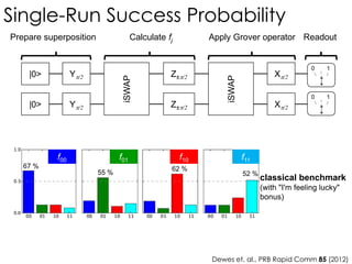
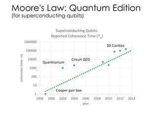
![|0>
|0>
Y/2
Y/2
iSWAP
Z-/2
Z-/2
iSWAP
X/2
X/2
Readout
0 1
0 1
Y(/2)
readout
50 100 150 200 ns
f01[f(t)],a(t)
0
iSWAP iSWAP
Z(/2)
X(/2)
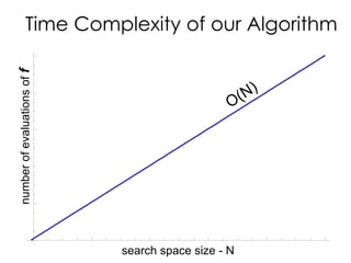
Running Grover-Search for 2 Qubits
Calculate fj Apply Grover operator
40
Prepare superposition](https://image.slidesharecdn.com/presentationhandout-141230060346-conversion-gate01/85/Let-s-build-a-quantum-computer-40-320.jpg)


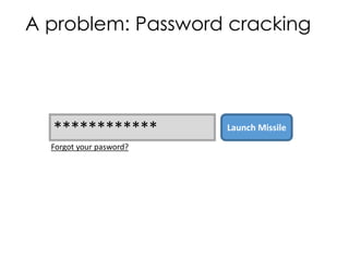
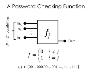
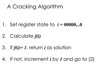
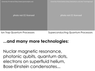
The document discusses the fundamentals and motivation behind quantum computing, highlighting its potential advantages over classical computing, particularly in tasks like password cracking. It outlines various quantum algorithms, including Grover's algorithm for search efficiency, and provides insights into building quantum processors using technologies like superconductors and ion traps. Despite advancements, the document notes significant engineering challenges that remain, suggesting that control of quantum computing may eventually lie with governments and corporations.


![Polymer [ बहुलक ] Chemistry Notes PDF - Irfanullah Mehar - JJ Sir Chemistry.pdf](https://cdn.slidesharecdn.com/ss_thumbnails/polymerchemistrynotespdf-irfanullahmehar-jjsirchemistry-260210172118-3f9b37f7-thumbnail.jpg?width=640&height=640&fit=bounds)


