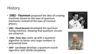
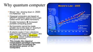
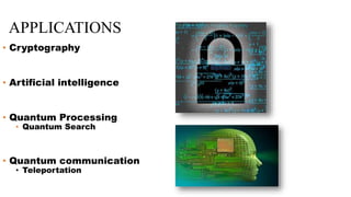
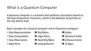
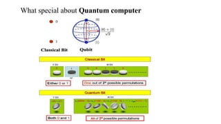
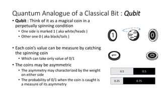
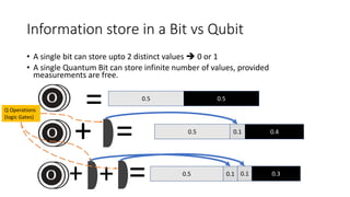
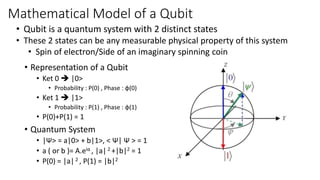
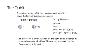
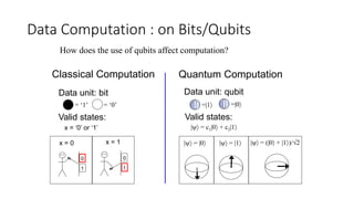
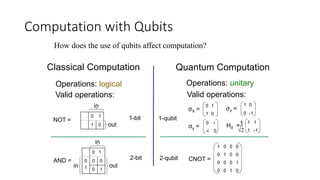
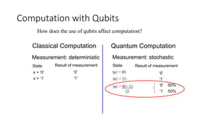
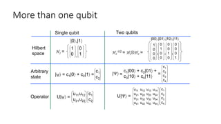
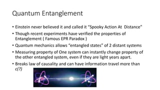
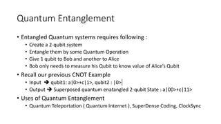
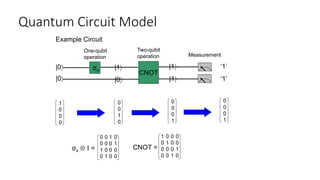
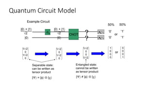
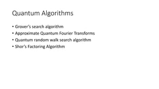
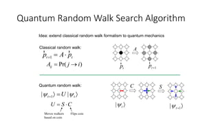
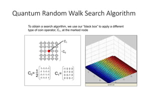
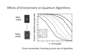
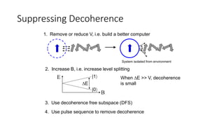
Quantum Computation
Prasenjit
Principal Engineering Manager@Microsoft
Nobody understands quantum
mechanics
“No, you’re not going to be able to understand it. . . .
You see, my physics students don’t understand it
either. That is because I don’t understand it. Nobody
does. ... The theory of quantum electrodynamics
describes Nature as absurd from the point of view of
common sense. And it agrees fully with an
experiment. So I hope that you can accept Nature as
She is -- absurd.”
Richard Feynman
Absurd : Yes, but works perfect as per those very
absurd equations and laws which governs them!!!
Agenda
• Introduction to Quantum Computation
• Brief History and Need of Quantum Computing
• Quantum Computing concepts
• Comparison with Classical Computing
• Qubits
• Quantum Logic Gates
• Quantum Circuits
• Quantum Programming
• Quantum Hello World
• Quantum Algorithms
History
 1982 - Feynman proposed the idea of creating
machines based on the laws of quantum
mechanics instead of the laws of classical
physics.
 1985 - David Deutsch developed the quantum
Turing machine, showing that quantum circuits
are universal.
 1994 - Peter Shor came up with a quantum
algorithm to factor very large numbers in
polynomial time.
 1997 - Lov Grover develops a quantum search
algorithm with O(√N) complexity
Why quantum computer
 Moore’ law slowing down in 2020
it is flattened out.
 Classical computers are based on
ON/OFF switches used to form Logic
Gates which are called transistors.
 Smaller transistors  Increased
portable computing power
 But transistor cannot be made
smaller due to the laws of Quantum
Mechanics starts to take over.
 At atomic scale (<1nm ) electrons
pass through closed logic gates ( aka
OFF switches ) due to Quantum
Tunneling, which nullifies presence
of Logical switches.
 This breaks the classical
computation paradigm and holds
us back from increasing the
computation power of our
Computers.
APPLICATIONS
• Cryptography
• Artificial intelligence
• Quantum Processing
• Quantum Search
• Quantum communication
• Teleportation
What is a Quantum Computer
A quantum computer is a machine that performs calculations based on
the laws of quantum mechanics, which is the behavior of particles at
the sub-atomic level.
Basic concepts of a classical computer and its Quantum analogues :
• Data Representation  Bits/Bytes Qubits
• Data Computation  Logic Gates  Quantum Gates
• Data Observation  Read Bits/Bytes Q Measurments
• Algorithms  Lookup/Search  Q Algos
What special about Quantum computer
Data Representation : The Bit
The basic component of a classical computer is the bit, a single
binary variable of value 0 or 1.
1
0
0
1
The state of a classical computer is described by some
long bit string of 0s and 1s.
0001010110110101000100110101110110...
At any given time, the value
of a bit is either ‘0’ or ‘1’.
Quantum Analogue of a Classical Bit : Qubit
• Qubit : Think of it as a magical coin in a
perpetually spinning condition
• One side is marked 1 ( aka white/heads )
• Other one 0 ( aka black/tails )
• Each coin’s value can be measure by catching
the spinning coin
• Which can take only value of 0/1
• The coins may be asymmetric
• The asymmetry may characterized by the weight
on either side
• The probability of 0/1 when the coin is caught is
a measure of its asymmetry
0.50.5
0.750.25
Information store in a Bit vs Qubit
• A single bit can store upto 2 distinct values  0 or 1
• A single Quantum Bit can store infinite number of values, provided
measurements are free.
0.1 0.40.5
+ =
+ 0.10.5
+ = 0.1
= 0.5 0.5
0.3
Q Operations
(logic Gates)
Mathematical Model of a Qubit
• Representation of a Qubit
• Ket 0  |0>
• Probability : P(0) , Phase : ɸ(0)
• Ket 1  |1>
• Probability : P(1) , Phase : ɸ(1)
• P(0)+P(1) = 1
• Quantum System
• |Ψ> = a|0> + b|1>, < Ψ| Ψ > = 1
• a ( or b )= A.eiα , |a|2 +|b|2 = 1
• P(0) = |a|2 , P(1) = |b|2
• Qubit is a quantum system with 2 distinct states
• These 2 states can be any measurable physical property of this system
• Spin of electron/Side of an imaginary spinning coin
The Qubit
A quantum bit, or qubit, is a two-state system which
obeys the laws of quantum mechanics.
=|1 =|0
Valid qubit states:
| = |0
| = |1
| = (|0- ei/4 |1)/2
| = (2|0- 3ei5/6 |1)/13
Spin-½ particle
The state of a qubit | can be thought of as a vector in
a two-dimensional Hilbert Space, H2, spanned by the
Basis vectors |0 and |1.
Data Computation : on Bits/Qubits
How does the use of qubits affect computation?
Classical Computation
Data unit: bit
x = 0 x = 1
0
1
0
1
Valid states:
x = ‘0’ or ‘1’ | = c1|0 + c2|1
Quantum Computation
Data unit: qubit
Valid states:
| = |0 | = |1 | = (|0 + |1)/√2
=|1 =|0= ‘1’ = ‘0’
Computation with Qubits
0 1
1 0
How does the use of qubits affect computation?
Classical Computation
Operations: logical
Valid operations:
AND =
0 i
-i 0
1 0
0 -1
1 1
1 -1
0 1
0
1
0 0
0 1
NOT =
0 1
1 0
in
out
out
in
in
1 0 0 0
0 1 0 0
0 0 0 1
0 0 1 0
1-bit
2-bit
Quantum Computation
Operations: unitary
Valid operations:
σX =
σy =
σz =
Hd =
CNOT =
√2
1
1-qubit
2-qubit
Computation with Qubits
How does the use of qubits affect computation?
Classical Computation
Measurement: deterministic
x = ‘0’
State Result of measurement
‘0’
x = ‘1’ ‘1’
Quantum Computation
Measurement: stochastic
| = |0
| = |0- |1
State Result of measurement
| = |1
2
‘0’
‘1’
‘0’ 50%
‘1’ 50%
More than one qubit
1
0
0
0
u11 u12
u21u22
Single qubit
c1
c2
c1
c2
Two qubits
H2 =
1
0
0
1,
|0,|1
H2
2 = H2H2 = ,
|00,|01,|10,|11
0
1
0
0
,
0
0
1
0
,
0
0
0
1
c1
c2
c3
c4
c1
c2
c3
c4
u11 u12 u13 u14
u21 u22 u23 u24
u31 u32 u33 u34
u41 u42 u43 u44
Hilbert
space
U| = U| =Operator
| = c1|0 + c2|1 = |
c1|00 + c2|01 +
c3|10 + c4|11
==
Arbitrary
state
Quantum Logic Gates ( 1 Qubit gates )
•NOT Gate
• |0  |1 and |1  |0
• Generalized Input state: c0|0 + c1|1
• Generalized Output state: c1|0 + c0|1
X0 1
1 0


 

0.1
= 0.9
+ = 0.9 0.1
0 
1
0


 

1 
0
1


 

Quantum Logic Gates ( 1 Qubit Gates )
• Hadamard Gate
• |0  1/√2 |0 + 1/√2 |1
• |1  1/√2 |0 – 1/√2 |1
1
2
1 1
1 1


 

H
1.0
=
0.50.5+ =
Advanced Computer Architecture Laboratory
• Controlled NOT (CNOT)
• Flips second Qubit iff the Control Qubit=1
• Quantum generalization of XOR Gate
• Input : a|00>+b|01>+c|10>+d|11>
• Output : a|00>+b|01>+d|10>+c|11>
• Specific Example :
• Let Qubit 1  a|0>+c|1>
• Let Qubit 2  |0>
• Input : a|00>+0|01>+ c|10>+0|11>
• Output : a|00>+0|01>+0|10>+c|11>
Quantum Gates ( 2 Qubit Gates)
1 0 0 0
0 1 0 0
0 0 0 1
0 0 1 0










Quantum Entanglement
• Einstein never believed it and called it “Spooky Action At Distance”
• Though recent experiments have verified the properties of
Entanglement ( Famous EPR Paradox )
• Quantum mechanics allows “entangled states” of 2 distant systems
• Measuring property of One system can instantly change property of
the other entangled system, even if they are light years apart.
• Breaks law of causality and can have information travel more than
c(?)
Quantum Entanglement
• Entangled Quantum systems requires following :
• Create a 2-qubit system
• Entangle them by some Quantum Operation
• Give 1 qubit to Bob and another to Alice
• Bob only needs to measure his Qubit to know value of Alice’s Qubit
• Recall our previous CNOT Example
• Input  qubit1: a|0>+c|1>, qubit2 : |0>
• Output  Superposed quantum enatangled 2-qubit State : a|00>+c|11>
• Uses of Quantum Entanglement
• Quantum Teleportation ( Quantum Internet ), SuperDense Coding, ClockSync
Quantum Circuit Model
1
0
0
0
0 0 1 0
0 0 0 1
1 0 0 0
0 1 0 0
σx  I =
0
0
1
0
1 0 0 0
0 1 0 0
0 0 0 1
0 0 1 0
CNOT =
0
0
0
1
0
0
0
1
|0
|0
|1
|0
|1
|1
‘1’
‘1’
Example Circuit
σx
One-qubit
operation
CNOT
Two-qubit
operation Measurement
Quantum Circuit Model
1/√2
0
1/√2
0
1
0
0
0
σx
CNOT
|0 + |1
|0
Example Circuit
√2
______
1/√2
0
1/√2
0
1/√2
0
0
1/√2
0
0
0
1
|0 + |1
|0
√2
______
‘0’
‘0’
or
‘1’
‘1’
or
50% 50%
Separable state:
can be written as
tensor product
| = |  |
Entangled state:
cannot be written
as tensor product
| ≠ |  |
?
?
Quantum Algorithms
• Grover’s search algorithm
• Approximate Quantum Fourier Transforms
• Quantum random walk search algorithm
• Shor’s Factoring Algorithm
Application of Grovers Search Algorithm
• Grover’s algorithm can identify an item from a list of N elements in
• What’s this good for?
• Unstructured database search (virtual database)
• Search an usorted list
• breaking DES (Data Encryption Standard)
• SAT (Satisfyability of boolean formula)
• map coloring with 4 colors
 NO
Grover’s Search Algorithm
The best a classical computer
can do on average is N/2 queries.
1 Oracle
No
...
2 Oracle
No
3 Oracle
Yes
Classical computer
Oracle
1+2+3+... No+No+Yes+No+...
Quantum computer
Using Grover’s algorithm, a quantum computer can
find the answer in N queries!
Superposition over all N possible inputs.
Grovers Search
• Suppose you are given a large list of items. Among these items there
is one item with a unique property that we wish to locate; we will call
this one the winner . Think of each item in the list as a box of a
particular color. Say all items in the list are gray except the winner ,
which is pink.
• Classical Algorithm requires (N+1)/2 on an average
Grovers Search
• Initialize an n-qubit quantum system with equal amplitudes
• Steps :
• Take an n Qubit system
• Initialize them to all 0  1|0000…0>
• Apply Hadamard Transform on it
•
1
𝑁
|0….0> +
1
𝑁
|0….1> + ……2 𝑛 times
Grovers Algorithm : Oracle Transform
• Apply Quantum Oracle transform
• The Quantum Oracle does following
• Flips the sign of the solution state
• Keeps others unchanged
•
1
𝑁
|0….0> +
1
𝑁
|0….1> -
1
𝑁
|1.0…>……
+….
• X  -X ( if X is the solution ), X
otherwise
Grovers Algorithm ( Amplitude Amplification )
• Now Perform diffusion transform
• It increases the amplitude by their
differences from the average,
decreasing if their difference is
negative
• Quantum Operator
• 2|Ψ><Ψ|-I
• Keep doing it multiple times
• Measure. Measured value is
your solution.
Grover’s Search Algorithm
Pros:
Can be used on any unstructured search problem, even
NP-complete problems.
Cons:
Only a quadratic speed-up over classical search.
O
σz
O
σz
…
…
…
…
|0
|0
|0
O(N) iterations
Hd
Hd
Hd
…Hd
Hd
Hd
…
Hd
Hd
Hd
…
Hd
Hd
Hd
…
Hd
Hd
Hd
NKS 2008
Does biological computation use quantum
searching?
• Mystery – DNA computation in cells uses an alphabet
of size 4 and protein synthesis uses an alphabet of
size 20 (20 amino acids).
• Observation – (Apoorva Patel, 2000) – Quantum
searching is most efficient when carried out for
databases of size:
4 - (requires 1 query)
10 - (requires 2 queries)
20 – ( requires 3 queries)
NKS 2008
h
Spatial Quantum Searching
• Quantum search type
algorithms can be used to
search a distributed
database using only
neighbor to neighbor
communications.with a
square-root speedup
over a classical database.
(Aaronson 2001)
Spatial Quantum Searching
• A robot needs to go to one marked
cell in a multidimensional array of N
items.
• A classical robot will need O(N)
steps to find and reach the marked
cell.
• A quantum robot will need only
O(√N) steps
NKS 2008
h
NKS 2008
h
ONsteps
h
O√Nsteps
NKS 2008
Photosynthesis
• Photosynthesis in plants is extremely efficient – unlike other chemical
& biological reactions, it is able to transport almost 100% of the
photons to the desired locations.
• This used to be a mystery – one possible explanation was given by
Fleming et al (Nature – April 14, 2007) where they analyzed the way
the energy flows in the cells as a spatial quantum search problem.
Does Nature use Quantum Searching?
Original algorithm - Database search & function inversion
Applications:
• Collision problem & Element Distinctness
• Communication algorithms
• Precision Measurements
• Pendulum Modes
Natural applications
• Genetic Pattern Matching (??)
• Photosynthesis (??)
Quantum Random Walk Search Algorithm
Idea: extend classical random walk formalism to quantum mechanics
A
tp
r
1tp 
r
Classical random walk:
C S
| t  1| t  
Quantum random walk:
1| |t tU    
U S C 
Moves walkers
based on coin
Flips coin
Pr( )ijA j i 
1t tp A p  
r r
Quantum Random Walk Search Algorithm
To obtain a search algorithm, we use our “black box” to apply a different
type of coin operator, C1, at the marked node
C0
C1
1 -1-1 -1
-1 1 -1 -1
-1 -1 1 -1
-1 -1-1 1
C0=
1
2
C1=
-1 0 0 0
0 -1 0 0
0 0 -1 0
0 0 0 -1
Quantum Random Walk Search Algorithm
Pros:
As general as Grover’s search algorithm.
Cons:
Same complexity as Grover’s search algorithm.
Slightly more complicated in implementation
Slightly more memory used
Interesting Feature: Search algorithm flows naturally
out of random walk formalism. Motivation for new QRW-
based algorithms?
Quantum Hello World
Quantum Hello World
• https://docs.microsoft.com/en-us/quantum/quantum-
installconfig?view=qsharp-preview
Q & A
Appendix
Decoherence and Noise
What happens to a qubit when it interacts with an environment?
0
0 1,
1
z
j j
j
H H V
H B
V A

 
 

 
r r
Quantum computer Environment
V
Quantum information is lost through decoherence.
σ1
σ2 σ3
σN…
Types of Decoherence
T1 processes: longitudinal relaxation, energy is lost to the environment
V
T2 processes: transverse relaxation, system becomes entangled with
the environment
V
+
+
What are the effects of decoherence?
Effects of Environment on Quantum Memory
Fidelity of stored information decays with time.
T1 – timescale of
longitudinal relaxation
T2 – timescale of
transverse relaxation
Effects of Environment on Quantum Algorithms
Errors accumulate, lowering success rate of algorithm
Grover’salgorithmsuccessrate
n = # of qubits
O
O
Ideal
oracle
Noisy
oracle
Suppressing Decoherence
1. Remove or reduce V, i.e. build a better computer
System isolated from environment
2. Increase B, i.e. increase level splitting
B
E
|0
|1 When E >> V, decoherence
is smallE
3. Use decoherence free subspace (DFS)
4. Use pulse sequence to remove decoherence

Quantum Computation For AI

  • 1.
  • 2.
    Nobody understands quantum mechanics “No,you’re not going to be able to understand it. . . . You see, my physics students don’t understand it either. That is because I don’t understand it. Nobody does. ... The theory of quantum electrodynamics describes Nature as absurd from the point of view of common sense. And it agrees fully with an experiment. So I hope that you can accept Nature as She is -- absurd.” Richard Feynman Absurd : Yes, but works perfect as per those very absurd equations and laws which governs them!!!
  • 3.
    Agenda • Introduction toQuantum Computation • Brief History and Need of Quantum Computing • Quantum Computing concepts • Comparison with Classical Computing • Qubits • Quantum Logic Gates • Quantum Circuits • Quantum Programming • Quantum Hello World • Quantum Algorithms
  • 4.
    History  1982 -Feynman proposed the idea of creating machines based on the laws of quantum mechanics instead of the laws of classical physics.  1985 - David Deutsch developed the quantum Turing machine, showing that quantum circuits are universal.  1994 - Peter Shor came up with a quantum algorithm to factor very large numbers in polynomial time.  1997 - Lov Grover develops a quantum search algorithm with O(√N) complexity
  • 5.
    Why quantum computer Moore’ law slowing down in 2020 it is flattened out.  Classical computers are based on ON/OFF switches used to form Logic Gates which are called transistors.  Smaller transistors  Increased portable computing power  But transistor cannot be made smaller due to the laws of Quantum Mechanics starts to take over.  At atomic scale (<1nm ) electrons pass through closed logic gates ( aka OFF switches ) due to Quantum Tunneling, which nullifies presence of Logical switches.  This breaks the classical computation paradigm and holds us back from increasing the computation power of our Computers.
  • 6.
    APPLICATIONS • Cryptography • Artificialintelligence • Quantum Processing • Quantum Search • Quantum communication • Teleportation
  • 7.
    What is aQuantum Computer A quantum computer is a machine that performs calculations based on the laws of quantum mechanics, which is the behavior of particles at the sub-atomic level. Basic concepts of a classical computer and its Quantum analogues : • Data Representation  Bits/Bytes Qubits • Data Computation  Logic Gates  Quantum Gates • Data Observation  Read Bits/Bytes Q Measurments • Algorithms  Lookup/Search  Q Algos
  • 8.
    What special aboutQuantum computer
  • 9.
    Data Representation :The Bit The basic component of a classical computer is the bit, a single binary variable of value 0 or 1. 1 0 0 1 The state of a classical computer is described by some long bit string of 0s and 1s. 0001010110110101000100110101110110... At any given time, the value of a bit is either ‘0’ or ‘1’.
  • 10.
    Quantum Analogue ofa Classical Bit : Qubit • Qubit : Think of it as a magical coin in a perpetually spinning condition • One side is marked 1 ( aka white/heads ) • Other one 0 ( aka black/tails ) • Each coin’s value can be measure by catching the spinning coin • Which can take only value of 0/1 • The coins may be asymmetric • The asymmetry may characterized by the weight on either side • The probability of 0/1 when the coin is caught is a measure of its asymmetry 0.50.5 0.750.25
  • 11.
    Information store ina Bit vs Qubit • A single bit can store upto 2 distinct values  0 or 1 • A single Quantum Bit can store infinite number of values, provided measurements are free. 0.1 0.40.5 + = + 0.10.5 + = 0.1 = 0.5 0.5 0.3 Q Operations (logic Gates)
  • 12.
    Mathematical Model ofa Qubit • Representation of a Qubit • Ket 0  |0> • Probability : P(0) , Phase : ɸ(0) • Ket 1  |1> • Probability : P(1) , Phase : ɸ(1) • P(0)+P(1) = 1 • Quantum System • |Ψ> = a|0> + b|1>, < Ψ| Ψ > = 1 • a ( or b )= A.eiα , |a|2 +|b|2 = 1 • P(0) = |a|2 , P(1) = |b|2 • Qubit is a quantum system with 2 distinct states • These 2 states can be any measurable physical property of this system • Spin of electron/Side of an imaginary spinning coin
  • 13.
    The Qubit A quantumbit, or qubit, is a two-state system which obeys the laws of quantum mechanics. =|1 =|0 Valid qubit states: | = |0 | = |1 | = (|0- ei/4 |1)/2 | = (2|0- 3ei5/6 |1)/13 Spin-½ particle The state of a qubit | can be thought of as a vector in a two-dimensional Hilbert Space, H2, spanned by the Basis vectors |0 and |1.
  • 14.
    Data Computation :on Bits/Qubits How does the use of qubits affect computation? Classical Computation Data unit: bit x = 0 x = 1 0 1 0 1 Valid states: x = ‘0’ or ‘1’ | = c1|0 + c2|1 Quantum Computation Data unit: qubit Valid states: | = |0 | = |1 | = (|0 + |1)/√2 =|1 =|0= ‘1’ = ‘0’
  • 15.
    Computation with Qubits 01 1 0 How does the use of qubits affect computation? Classical Computation Operations: logical Valid operations: AND = 0 i -i 0 1 0 0 -1 1 1 1 -1 0 1 0 1 0 0 0 1 NOT = 0 1 1 0 in out out in in 1 0 0 0 0 1 0 0 0 0 0 1 0 0 1 0 1-bit 2-bit Quantum Computation Operations: unitary Valid operations: σX = σy = σz = Hd = CNOT = √2 1 1-qubit 2-qubit
  • 16.
    Computation with Qubits Howdoes the use of qubits affect computation? Classical Computation Measurement: deterministic x = ‘0’ State Result of measurement ‘0’ x = ‘1’ ‘1’ Quantum Computation Measurement: stochastic | = |0 | = |0- |1 State Result of measurement | = |1 2 ‘0’ ‘1’ ‘0’ 50% ‘1’ 50%
  • 17.
    More than onequbit 1 0 0 0 u11 u12 u21u22 Single qubit c1 c2 c1 c2 Two qubits H2 = 1 0 0 1, |0,|1 H2 2 = H2H2 = , |00,|01,|10,|11 0 1 0 0 , 0 0 1 0 , 0 0 0 1 c1 c2 c3 c4 c1 c2 c3 c4 u11 u12 u13 u14 u21 u22 u23 u24 u31 u32 u33 u34 u41 u42 u43 u44 Hilbert space U| = U| =Operator | = c1|0 + c2|1 = | c1|00 + c2|01 + c3|10 + c4|11 == Arbitrary state
  • 18.
    Quantum Logic Gates( 1 Qubit gates ) •NOT Gate • |0  |1 and |1  |0 • Generalized Input state: c0|0 + c1|1 • Generalized Output state: c1|0 + c0|1 X0 1 1 0      0.1 = 0.9 + = 0.9 0.1 0  1 0      1  0 1     
  • 19.
    Quantum Logic Gates( 1 Qubit Gates ) • Hadamard Gate • |0  1/√2 |0 + 1/√2 |1 • |1  1/√2 |0 – 1/√2 |1 1 2 1 1 1 1      H 1.0 = 0.50.5+ =
  • 20.
    Advanced Computer ArchitectureLaboratory • Controlled NOT (CNOT) • Flips second Qubit iff the Control Qubit=1 • Quantum generalization of XOR Gate • Input : a|00>+b|01>+c|10>+d|11> • Output : a|00>+b|01>+d|10>+c|11> • Specific Example : • Let Qubit 1  a|0>+c|1> • Let Qubit 2  |0> • Input : a|00>+0|01>+ c|10>+0|11> • Output : a|00>+0|01>+0|10>+c|11> Quantum Gates ( 2 Qubit Gates) 1 0 0 0 0 1 0 0 0 0 0 1 0 0 1 0          
  • 21.
    Quantum Entanglement • Einsteinnever believed it and called it “Spooky Action At Distance” • Though recent experiments have verified the properties of Entanglement ( Famous EPR Paradox ) • Quantum mechanics allows “entangled states” of 2 distant systems • Measuring property of One system can instantly change property of the other entangled system, even if they are light years apart. • Breaks law of causality and can have information travel more than c(?)
  • 22.
    Quantum Entanglement • EntangledQuantum systems requires following : • Create a 2-qubit system • Entangle them by some Quantum Operation • Give 1 qubit to Bob and another to Alice • Bob only needs to measure his Qubit to know value of Alice’s Qubit • Recall our previous CNOT Example • Input  qubit1: a|0>+c|1>, qubit2 : |0> • Output  Superposed quantum enatangled 2-qubit State : a|00>+c|11> • Uses of Quantum Entanglement • Quantum Teleportation ( Quantum Internet ), SuperDense Coding, ClockSync
  • 23.
    Quantum Circuit Model 1 0 0 0 00 1 0 0 0 0 1 1 0 0 0 0 1 0 0 σx  I = 0 0 1 0 1 0 0 0 0 1 0 0 0 0 0 1 0 0 1 0 CNOT = 0 0 0 1 0 0 0 1 |0 |0 |1 |0 |1 |1 ‘1’ ‘1’ Example Circuit σx One-qubit operation CNOT Two-qubit operation Measurement
  • 24.
    Quantum Circuit Model 1/√2 0 1/√2 0 1 0 0 0 σx CNOT |0+ |1 |0 Example Circuit √2 ______ 1/√2 0 1/√2 0 1/√2 0 0 1/√2 0 0 0 1 |0 + |1 |0 √2 ______ ‘0’ ‘0’ or ‘1’ ‘1’ or 50% 50% Separable state: can be written as tensor product | = |  | Entangled state: cannot be written as tensor product | ≠ |  | ? ?
  • 25.
    Quantum Algorithms • Grover’ssearch algorithm • Approximate Quantum Fourier Transforms • Quantum random walk search algorithm • Shor’s Factoring Algorithm
  • 26.
    Application of GroversSearch Algorithm • Grover’s algorithm can identify an item from a list of N elements in • What’s this good for? • Unstructured database search (virtual database) • Search an usorted list • breaking DES (Data Encryption Standard) • SAT (Satisfyability of boolean formula) • map coloring with 4 colors  NO
  • 27.
    Grover’s Search Algorithm Thebest a classical computer can do on average is N/2 queries. 1 Oracle No ... 2 Oracle No 3 Oracle Yes Classical computer Oracle 1+2+3+... No+No+Yes+No+... Quantum computer Using Grover’s algorithm, a quantum computer can find the answer in N queries! Superposition over all N possible inputs.
  • 28.
    Grovers Search • Supposeyou are given a large list of items. Among these items there is one item with a unique property that we wish to locate; we will call this one the winner . Think of each item in the list as a box of a particular color. Say all items in the list are gray except the winner , which is pink. • Classical Algorithm requires (N+1)/2 on an average
  • 29.
    Grovers Search • Initializean n-qubit quantum system with equal amplitudes • Steps : • Take an n Qubit system • Initialize them to all 0  1|0000…0> • Apply Hadamard Transform on it • 1 𝑁 |0….0> + 1 𝑁 |0….1> + ……2 𝑛 times
  • 30.
    Grovers Algorithm :Oracle Transform • Apply Quantum Oracle transform • The Quantum Oracle does following • Flips the sign of the solution state • Keeps others unchanged • 1 𝑁 |0….0> + 1 𝑁 |0….1> - 1 𝑁 |1.0…>…… +…. • X  -X ( if X is the solution ), X otherwise
  • 31.
    Grovers Algorithm (Amplitude Amplification ) • Now Perform diffusion transform • It increases the amplitude by their differences from the average, decreasing if their difference is negative • Quantum Operator • 2|Ψ><Ψ|-I • Keep doing it multiple times • Measure. Measured value is your solution.
  • 32.
    Grover’s Search Algorithm Pros: Canbe used on any unstructured search problem, even NP-complete problems. Cons: Only a quadratic speed-up over classical search. O σz O σz … … … … |0 |0 |0 O(N) iterations Hd Hd Hd …Hd Hd Hd … Hd Hd Hd … Hd Hd Hd … Hd Hd Hd
  • 33.
    NKS 2008 Does biologicalcomputation use quantum searching? • Mystery – DNA computation in cells uses an alphabet of size 4 and protein synthesis uses an alphabet of size 20 (20 amino acids). • Observation – (Apoorva Patel, 2000) – Quantum searching is most efficient when carried out for databases of size: 4 - (requires 1 query) 10 - (requires 2 queries) 20 – ( requires 3 queries)
  • 34.
    NKS 2008 h Spatial QuantumSearching • Quantum search type algorithms can be used to search a distributed database using only neighbor to neighbor communications.with a square-root speedup over a classical database. (Aaronson 2001)
  • 35.
    Spatial Quantum Searching •A robot needs to go to one marked cell in a multidimensional array of N items. • A classical robot will need O(N) steps to find and reach the marked cell. • A quantum robot will need only O(√N) steps NKS 2008 h NKS 2008 h ONsteps h O√Nsteps
  • 36.
    NKS 2008 Photosynthesis • Photosynthesisin plants is extremely efficient – unlike other chemical & biological reactions, it is able to transport almost 100% of the photons to the desired locations. • This used to be a mystery – one possible explanation was given by Fleming et al (Nature – April 14, 2007) where they analyzed the way the energy flows in the cells as a spatial quantum search problem.
  • 37.
    Does Nature useQuantum Searching? Original algorithm - Database search & function inversion Applications: • Collision problem & Element Distinctness • Communication algorithms • Precision Measurements • Pendulum Modes Natural applications • Genetic Pattern Matching (??) • Photosynthesis (??)
  • 38.
    Quantum Random WalkSearch Algorithm Idea: extend classical random walk formalism to quantum mechanics A tp r 1tp  r Classical random walk: C S | t  1| t   Quantum random walk: 1| |t tU     U S C  Moves walkers based on coin Flips coin Pr( )ijA j i  1t tp A p   r r
  • 39.
    Quantum Random WalkSearch Algorithm To obtain a search algorithm, we use our “black box” to apply a different type of coin operator, C1, at the marked node C0 C1 1 -1-1 -1 -1 1 -1 -1 -1 -1 1 -1 -1 -1-1 1 C0= 1 2 C1= -1 0 0 0 0 -1 0 0 0 0 -1 0 0 0 0 -1
  • 40.
    Quantum Random WalkSearch Algorithm Pros: As general as Grover’s search algorithm. Cons: Same complexity as Grover’s search algorithm. Slightly more complicated in implementation Slightly more memory used Interesting Feature: Search algorithm flows naturally out of random walk formalism. Motivation for new QRW- based algorithms?
  • 41.
  • 42.
    Quantum Hello World •https://docs.microsoft.com/en-us/quantum/quantum- installconfig?view=qsharp-preview
  • 43.
  • 44.
  • 45.
    Decoherence and Noise Whathappens to a qubit when it interacts with an environment? 0 0 1, 1 z j j j H H V H B V A         r r Quantum computer Environment V Quantum information is lost through decoherence. σ1 σ2 σ3 σN…
  • 46.
    Types of Decoherence T1processes: longitudinal relaxation, energy is lost to the environment V T2 processes: transverse relaxation, system becomes entangled with the environment V + + What are the effects of decoherence?
  • 47.
    Effects of Environmenton Quantum Memory Fidelity of stored information decays with time. T1 – timescale of longitudinal relaxation T2 – timescale of transverse relaxation
  • 48.
    Effects of Environmenton Quantum Algorithms Errors accumulate, lowering success rate of algorithm Grover’salgorithmsuccessrate n = # of qubits O O Ideal oracle Noisy oracle
  • 49.
    Suppressing Decoherence 1. Removeor reduce V, i.e. build a better computer System isolated from environment 2. Increase B, i.e. increase level splitting B E |0 |1 When E >> V, decoherence is smallE 3. Use decoherence free subspace (DFS) 4. Use pulse sequence to remove decoherence