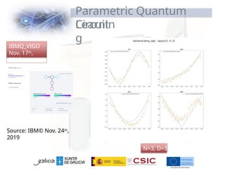
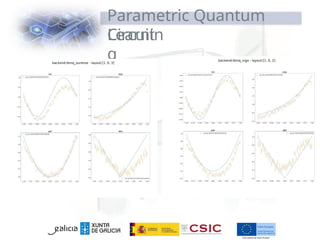
Schedule
2
Lecture 1:Introduction to Quantum
Computing.
My First Quantum Program.
Lecture 2: Programming Quantum
Algorithms
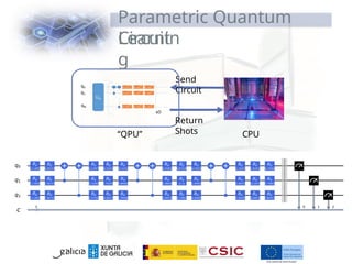
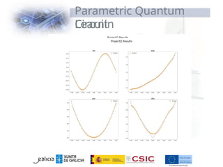
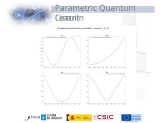
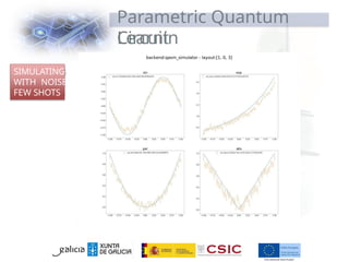
My first Quantum Program with ProjectQ
Lecture 3: Basic Quantum algorithms
Lecture 4: Advanced algorithms
3.
Lecture 1
Abrief history of QC and
needs. Types of quantum
computers.
Basic concepts: qubit,
tensors, multiqubit,
quantum gates,
measurement, amplitudes
My first quantum program.
Quantum Circuits. Width,
Depth, Quantum Volume.
4.
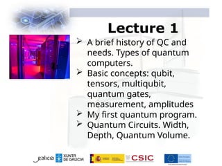
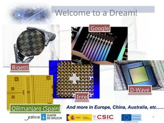
Welcome to aDream!
Yuri Manin (1980) and Richard Feynman (1981) proposed
independently the concept of Quantum Computer
I’m here very
“hot”!!
-273ºC
4
Source: IBM
https://en.wikipedia.org/wiki/Timeline_of_quantum_computing
5.
Welcome to aDream!
Rigetti
Intel
Google
D-Wave
Qilimanjaro (Spain) And more in Europe, China, Australia, etc……
5
6.
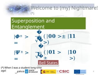
Welcome to (my)Nightmare!
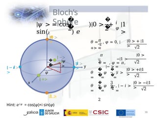
(*)
|𝜱± >
=
�
� ( 𝟎𝟎 >± 𝟏𝟏
>)
|𝜳± >
=
�
�
𝟏
�
�
( 𝟎𝟏 >
±
𝟏𝟎
>)
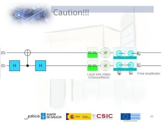
Bell States
Superposition and
Entanglement
6
(*) When I was a student long time
ago!
Quantum Computer
Quantumsimulator [1]. Simulate a quantum system using another one,
maybe simpler, that can be controlled by the experimenter.
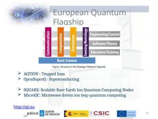
Adiabatic Quantum Computer [2]. Prepares a known and easy
Hamiltonian and lets it evolve to solution.
Topological Quantum Computer[4]. Uses topological properties.
Continuous Variable Quantum Computer [5].
Universal Quantum Computer [3].
1Reviewed in Georgescu, I. M., Ashhab, S., & Nori, F. (2014). Quantum simulation. Reviews of Modern Physics, 86(1), 153–
185. http://doi.org/10.1103/RevModPhys.86.153 arXiv:1308.6253
2 Reviewed in Albash, T., & Lidar, D. A. (2016). Adiabatic Quantum Computing. arxiv:1611.04471
3Proposed in Deutsch, D. (1985). http://doi.org/10.1098/rspa.1985.0070
and Deutsch, D. (1989). http://doi.org/10.1098/rspa.1989.0099
4 Lahtinen V., Pachos J.K.. SciPost Phys. 3, 021 (2017) arXiv:1705.04103
5 Lloyd S. & Braunstein, A.L. Phys.Rev.Lett. 82 (1999) 1784-1787.
arXiv:quant-ph/9810082 11
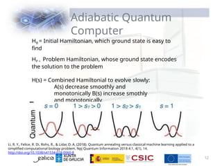
12.
Adiabatic Quantum
Computer
HB =Initial Hamiltonian, which ground state is easy to
find
HP = Problem Hamiltonian, whose ground state encodes
the solution to the problem
H(s) = Combined Hamiltonial to evolve slowly:
A(s) decrease smoothly and
monotonically B(s) increase smothly
and monotonically
H(s) = A(s)HB + B(s)HP
Li, R. Y., Felice, R. Di, Rohs, R., & Lidar, D. A. (2018). Quantum annealing versus classical machine learning applied to a
simplified computational biology problem. Npj Quantum Information 2018 4:1, 4(1), 14.
http://doi.org/10.1038/s41534-018-0060-8
12
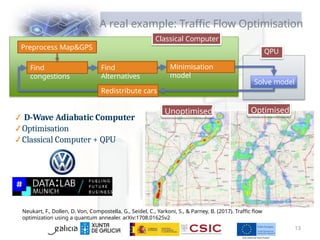
13.
A real example:Traffic Flow Optimisation
Neukart, F., Dollen, D. Von, Compostella, G., Seidel, C., Yarkoni, S., & Parney, B. (2017). Traffic flow
optimization using a quantum annealer. arXiv:1708.01625v2
D-Wave Adiabatic Computer
Optimisation
Classical Computer + QPU
Unoptimised Optimised
Preprocess Map&GPS
Find
congestions
Find
Alternatives
Minimisation
model
Solve model
Redistribute cars
Classical Computer
QPU
13
Lecture 1
Abrief history of QC and
needs. Types of quantum
computers.
Basic concepts: qubit,
tensors, multiqubit, quantum
gates, measurement,
amplitudes
My first quantum program.
Quantum Circuits. Width,
Depth, Quantum Volume.
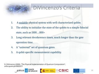
20.
1. A scalablephysical system with well characterized qubits.
2. The ability to initialize the state of the qubits to a simple fiducial
state, such as |000….000>
3. Long relevant decoherence times, much longer than the gate
operation time.
4. A “universal” set of quantum gates.
5. A qubit-specific measurement capability.
20
DiVincenzo’s Criteria
D. DiVincenzo (2000). “The Physical Implementation of Quantum Computation“,
arXiv:quant-ph/0002077
21.
What do youneed (today)?
21
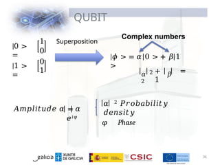
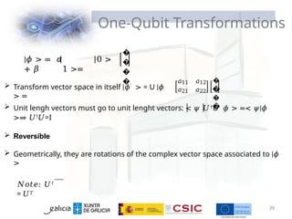
Complex numbers
Matrix multiplication
Understand TENSOR products
Understand measurement and probabilities
Imagination
22.
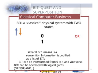
BIT, QUBIT AND
SUPERPOSITION
BIT:A “classical” physical system with TWO
states
0 OR
1
What 0 or 1 means is a
convention Information is codified
as a list of BITs
BIT can be transformed from 0 to 1 and vice versa
BITs can be operated with logical gates
(OR,XOR,AND…)
One BIT can be
Classical Computer Business
Card
22
23.
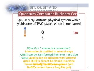
BIT, QUBIT AND
SUPERPOSITION
QuantumComputer Business Card
QuBIT: A “Quantum” physical system which
yields one of TWO states when is measured
0 OR
1
What 0 or 1 means is a convention*
Information is codified in several ways
QuBIT can be transformed from 0 to 1 and vice
versa QuBITs can be operated with UNITARY
gates QuBITs cannot be cloned (no-clone
theorem) QuBITs cannot be stored (yet)
QuBITs cannot have a long life (yet)
Usually, QuBITs are quiet
23
24.
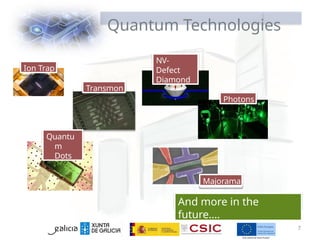
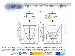
Quantum Technologies
Krantz P,Kjaergaard M, Yan F, Orlando TP, Gustavsson S, Oliver WD. A
Quantum Engineer’s Guide to Superconducting Qubits. Arxiv: 1904.06560
www.inl.int
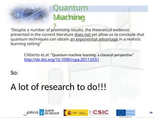
“Despite a numberof promising results, the theoretical evidence
presented in the current literature does not yet allow us to conclude that
quantum techniques can obtain an exponential advantage in a realistic
learning setting”
Ciliberto et.al. “Quantum machine learning: a classical perspective”
http://dx.doi.org/10.1098/rspa.2017.0551
34
Quantum
Machine
Learning
?
So:
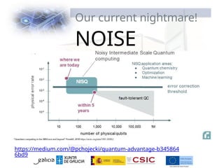
A lot of research to do!!!
35.
www.inl.int
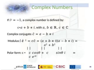
Complex Numbers
If 𝑖2= −1, a complex number is defined by:
c=𝑎 + 𝑏 ∗ 𝑖, with 𝑎, 𝑏 ∈ ℝ, 𝑐 ∈ ℂ
Complex conjugate: 𝑐̅ = 𝑎 − 𝑏 ∗ 𝑖
Modulus: 𝑐 2 = 𝑐𝑐̅ = (𝑎 + 𝑏 ∗ 𝑖)(𝑎 − 𝑏 ∗ 𝑖) =
𝑎2 + 𝑏2
Polar form: c = 𝑐 𝑐𝑜𝑠𝜃 + 𝑐 𝑠𝑖𝑛𝜃 𝑖 =
𝑐 𝑒𝑖𝜃
35
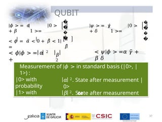
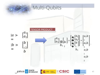
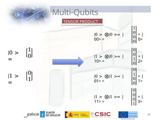
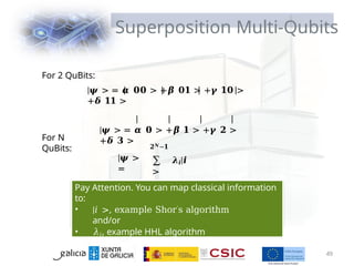
Superposition Multi-Qubits
For N
QuBits:
For2 QuBits:
|𝝍 > = 𝜶 𝟎𝟎 > +𝜷 𝟎𝟏 > +𝜸 𝟏𝟎 >
+𝜹 𝟏𝟏 >
|𝝍 > = 𝜶 𝟎 > +𝜷 𝟏 > +𝜸 𝟐 >
+𝜹 𝟑 >
|𝝍 >
=
𝟐𝑵−𝟏
∑ 𝝀𝒊|𝒊
>
𝒊=𝟎
Pay Attention. You can map classical information
to:
• |𝑖 >, example Shor′s algorithm
and/or
• 𝜆𝑖, example HHL algorithm
49
48.
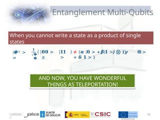
Entanglement Multi-Qubits
13/09/201
7
50
When youcannot write a state as a product of single
states
|𝜱± >
=
𝟏
�
�
𝟎𝟎 >
±
𝟏𝟏
>
≠ (𝜶 |𝟎 > +𝜷|𝟏 >) ⨂ (𝜸 𝟎 >
+ 𝜹 𝟏 > )
AND NOW, YOU HAVE WONDERFUL
THINGS AS TELEPORTATION!
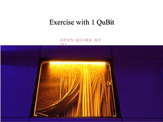
O P EN Q U I R K . H T
M L
MY FIRST QUANTUM
PROGRAM:
Superdense Coding
55.
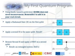
My First QuantumProgram
Using Quirk. Launch quirk.html. QUIRK does not
need measurement. Remember to add it in
your real circuit.
Apply a Hadamard Gate (H) on the first qubit
Apply a second H to the same qubit. Result?
Remove Second H and apply a CNOT on a second
qubit.
Result: an entangled system (Bell’s)
13/09/201
7
57
56.
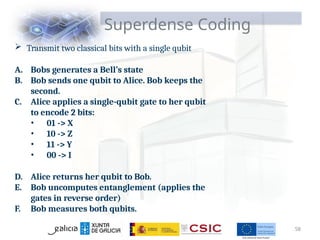
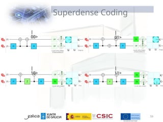
Superdense Coding
58
Transmittwo classical bits with a single qubit
A. Bobs generates a Bell’s state
B. Bob sends one qubit to Alice. Bob keeps the
second.
C. Alice applies a single-qubit gate to her qubit
to encode 2 bits:
• 01 -> X
• 10 -> Z
• 11 -> Y
• 00 -> I
D. Alice returns her qubit to Bob.
E. Bob uncomputes entanglement (applies the
gates in reverse order)
F. Bob measures both qubits.
C O NN E C T T O : H T T P S : / / Q U A N T U M - C O M P U T I N G . I
B M . C O M /
Exercise 2: IBM Quantum
Experience
60.
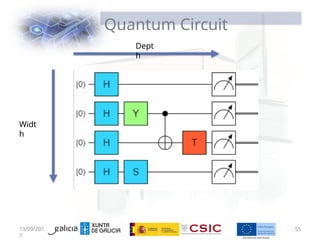
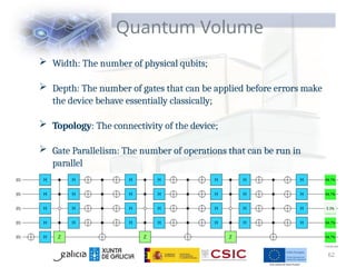
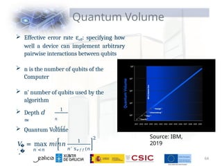
Quantum Volume
Width:The number of physical qubits;
Depth: The number of gates that can be applied before errors make
the device behave essentially classically;
Topology: The connectivity of the device;
Gate Parallelism: The number of operations that can be run in
parallel
62
Quantum Volume
Effectiveerror rate εeff: specifying how
well a device can implement arbitrary
pairwise interactions between qubits
n is the number of qubits of the
Computer
n’ number of qubits used by the
algorithm
Depth 𝑑
≃
1
𝑛
𝗌𝑒𝑓𝑓
Quantum Volume
�
� 𝑛′<𝑛
𝑉 = max 𝑚𝑖𝑛𝑛
′,
1
𝑛′ 𝗌𝑒𝑓𝑓(𝑛
′)
2 Source: IBM,
2019
64
How many states?
Asimovcalculated the number of
nucleons+electrons in the Universe as ∼1079
∼
10.000.000.000.000.000.000.000.000.000.000.000.000.000.000.000.000.000.000.000.000.000.0
00.000.000.000.000
Having a QPU with 270 qubits, one can store in
the amplitudes: ∼1081 FPs.
Year 2025: ∼170ZB/year ∼ 1023
bytes/year
75 qubits: ∼ 3·1023 FPs = ∼ 24
years!!!!
65.
Classical
Resources
qubits RAM
1 32bytes + memory for gates
2 64 bytes + memory for gates
3 128 bytes + memory for gates
4 256 bytes + memory for gates
8 4 kbytes + memory for gates
16 1 Mbytes + memory for gates
32 64 Gbytes + memory for gates
36 1TB + …..
38 4TB (Limit CESGA FT2 FAT node
….)
45 0,5PB [1]
64 512 ExaBytes!!!
THIS IS ONLY TRUE IF YOU NEED ALL POSSIBLE STATES!
[1] Häner, T., & Steiger, D. S. (2017). 0.5 Petabyte Simulation of a 45-Qubit Quantum Circuit. Arxiv:1704.01127
67
![Quantum Computer
Quantum simulator [1]. Simulate a quantum system using another one,
maybe simpler, that can be controlled by the experimenter.
Adiabatic Quantum Computer [2]. Prepares a known and easy
Hamiltonian and lets it evolve to solution.
Topological Quantum Computer[4]. Uses topological properties.
Continuous Variable Quantum Computer [5].
Universal Quantum Computer [3].
1Reviewed in Georgescu, I. M., Ashhab, S., & Nori, F. (2014). Quantum simulation. Reviews of Modern Physics, 86(1), 153–
185. http://doi.org/10.1103/RevModPhys.86.153 arXiv:1308.6253
2 Reviewed in Albash, T., & Lidar, D. A. (2016). Adiabatic Quantum Computing. arxiv:1611.04471
3Proposed in Deutsch, D. (1985). http://doi.org/10.1098/rspa.1985.0070
and Deutsch, D. (1989). http://doi.org/10.1098/rspa.1989.0099
4 Lahtinen V., Pachos J.K.. SciPost Phys. 3, 021 (2017) arXiv:1705.04103
5 Lloyd S. & Braunstein, A.L. Phys.Rev.Lett. 82 (1999) 1784-1787.
arXiv:quant-ph/9810082 11](https://image.slidesharecdn.com/qc-250501103645-60de8189/85/quantum-computing-presentation-for-professionals-11-320.jpg)
![Classical
Resources
qubits RAM
1 32 bytes + memory for gates
2 64 bytes + memory for gates
3 128 bytes + memory for gates
4 256 bytes + memory for gates
8 4 kbytes + memory for gates
16 1 Mbytes + memory for gates
32 64 Gbytes + memory for gates
36 1TB + …..
38 4TB (Limit CESGA FT2 FAT node
….)
45 0,5PB [1]
64 512 ExaBytes!!!
THIS IS ONLY TRUE IF YOU NEED ALL POSSIBLE STATES!
[1] Häner, T., & Steiger, D. S. (2017). 0.5 Petabyte Simulation of a 45-Qubit Quantum Circuit. Arxiv:1704.01127
67](https://image.slidesharecdn.com/qc-250501103645-60de8189/85/quantum-computing-presentation-for-professionals-65-320.jpg)