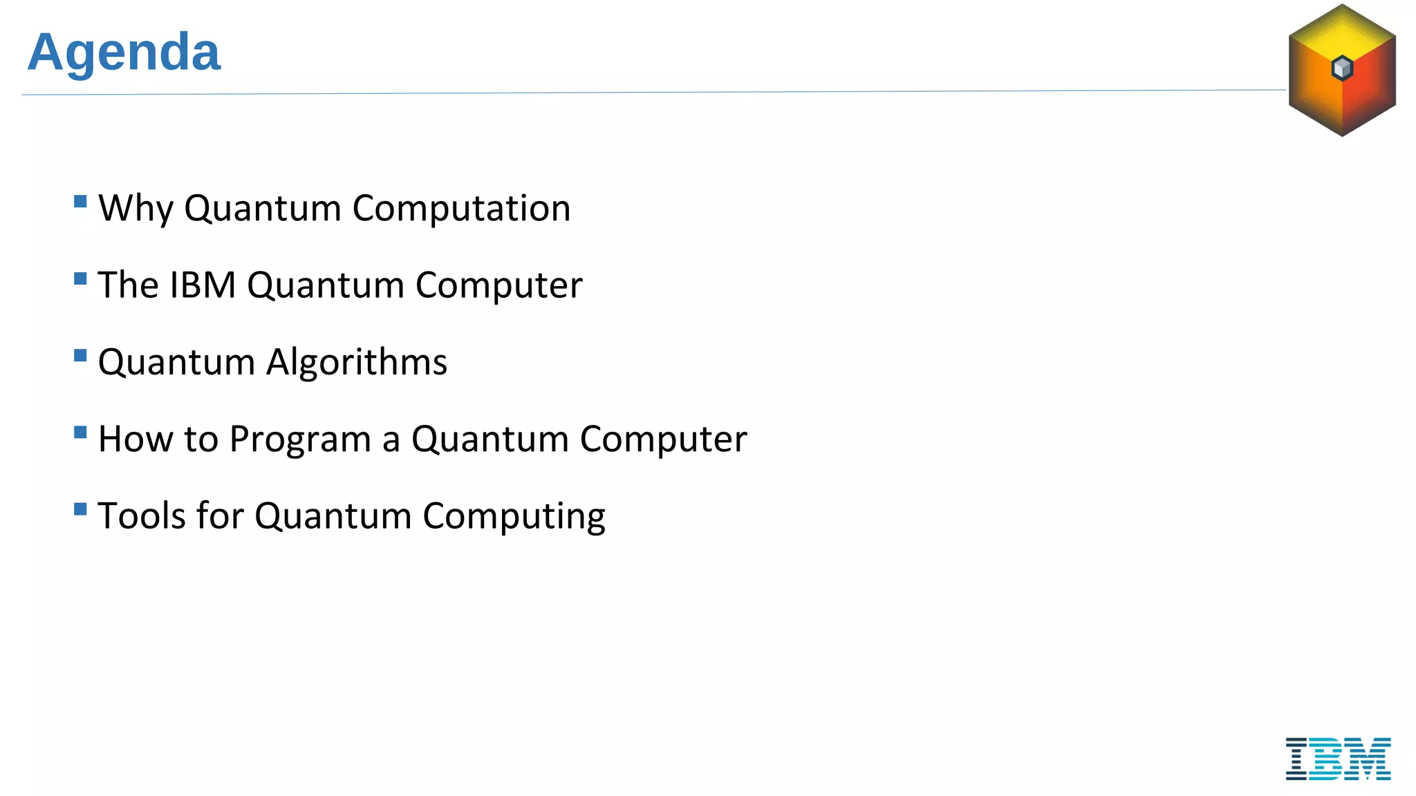
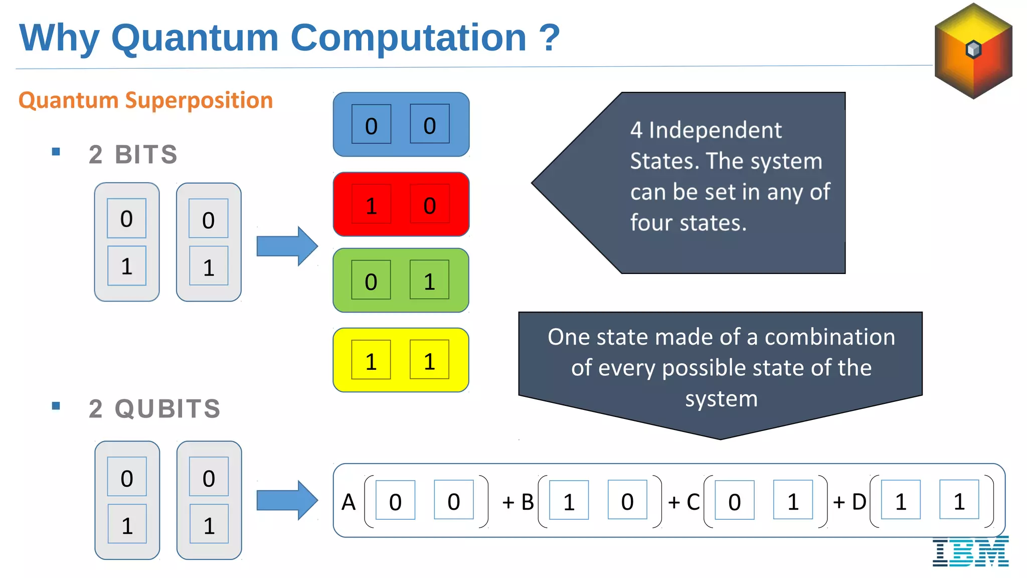
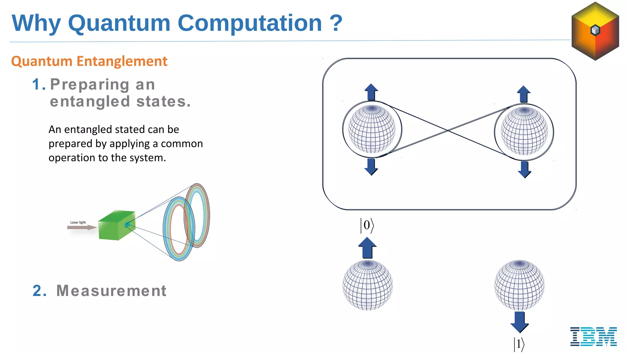
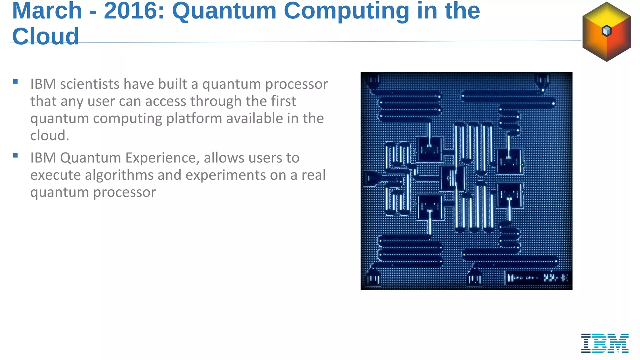
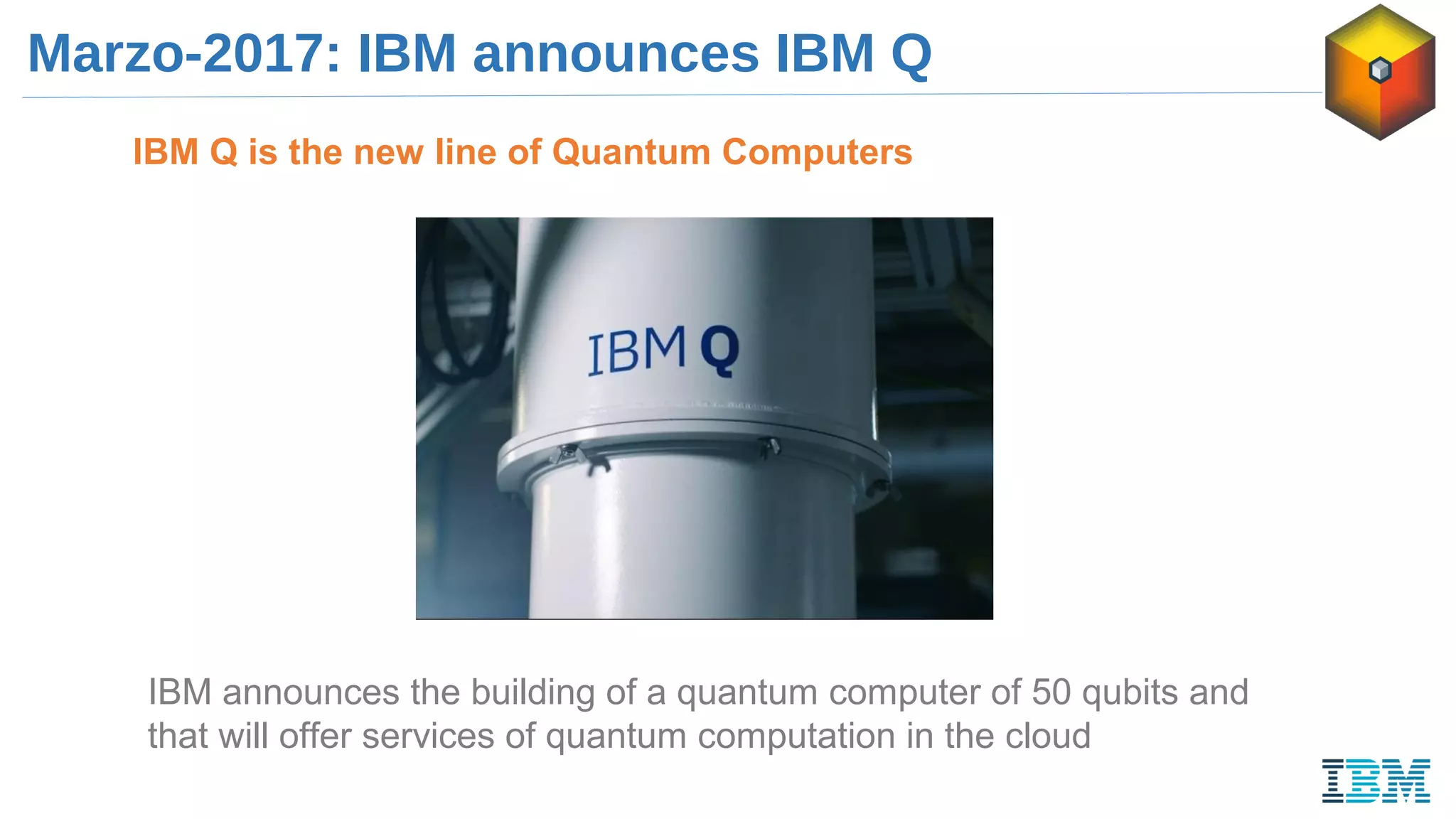
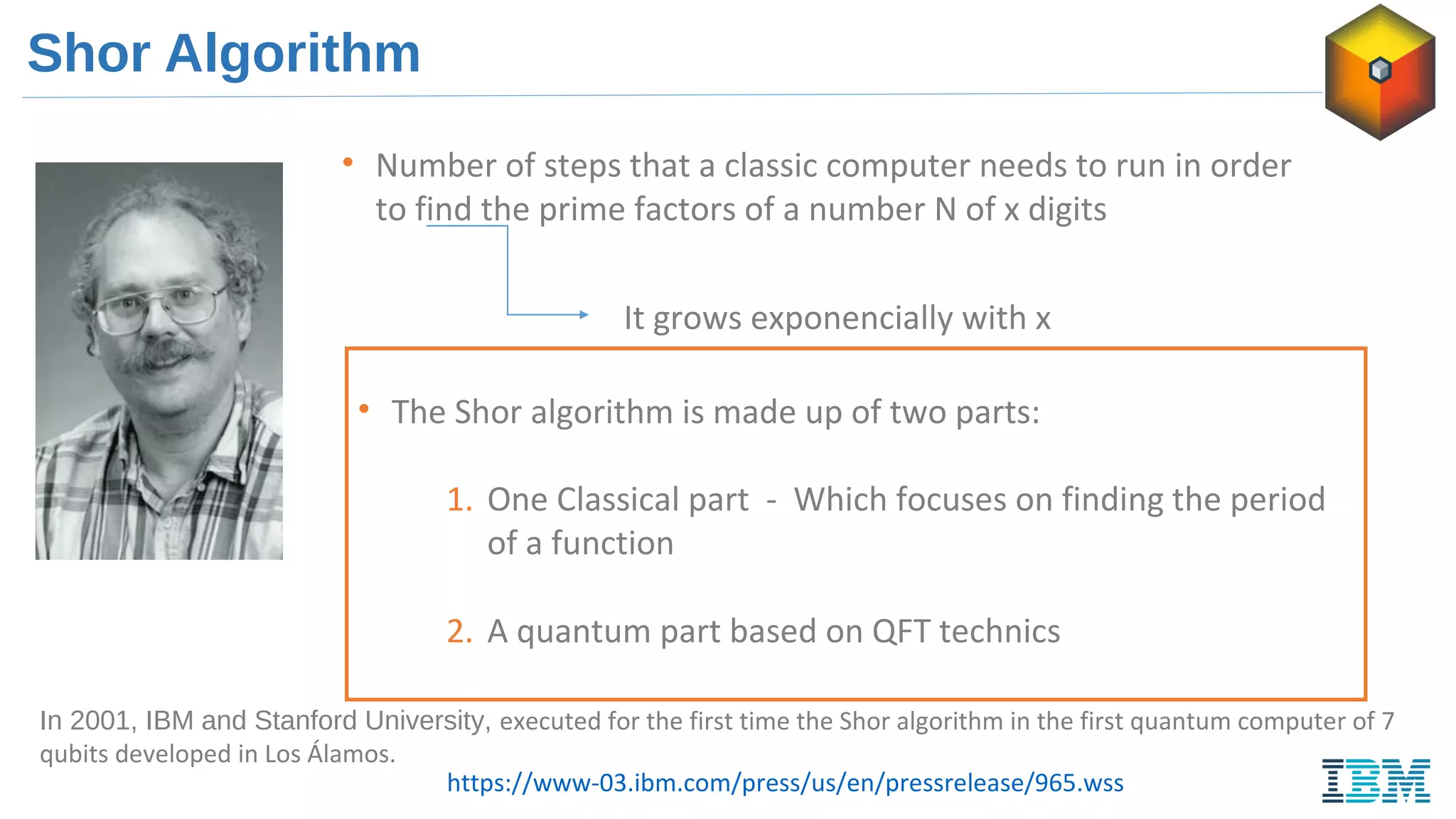
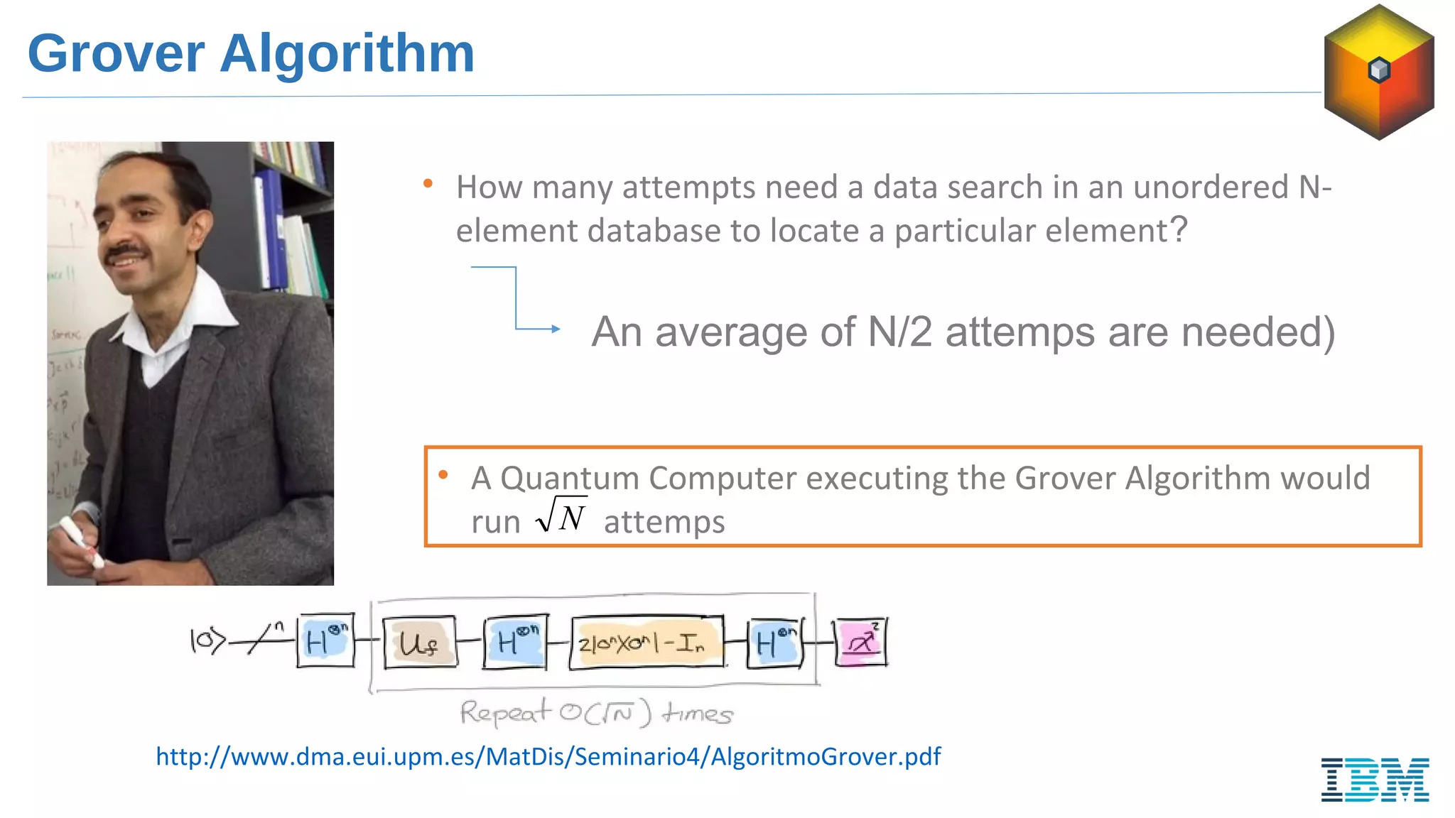
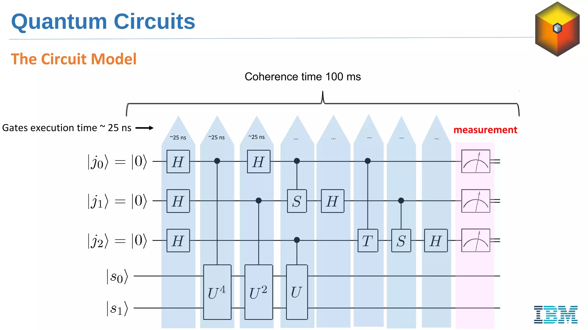
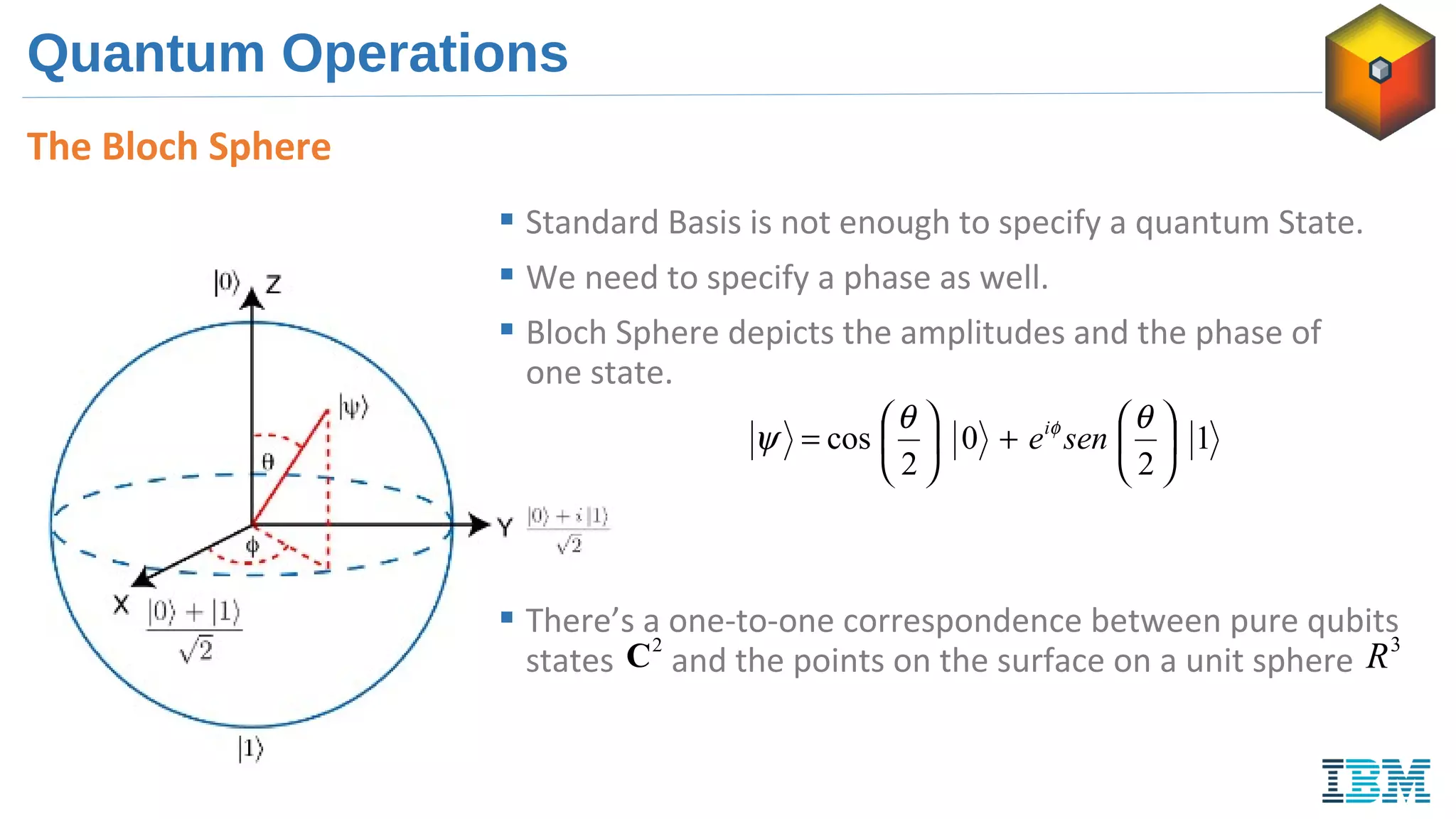
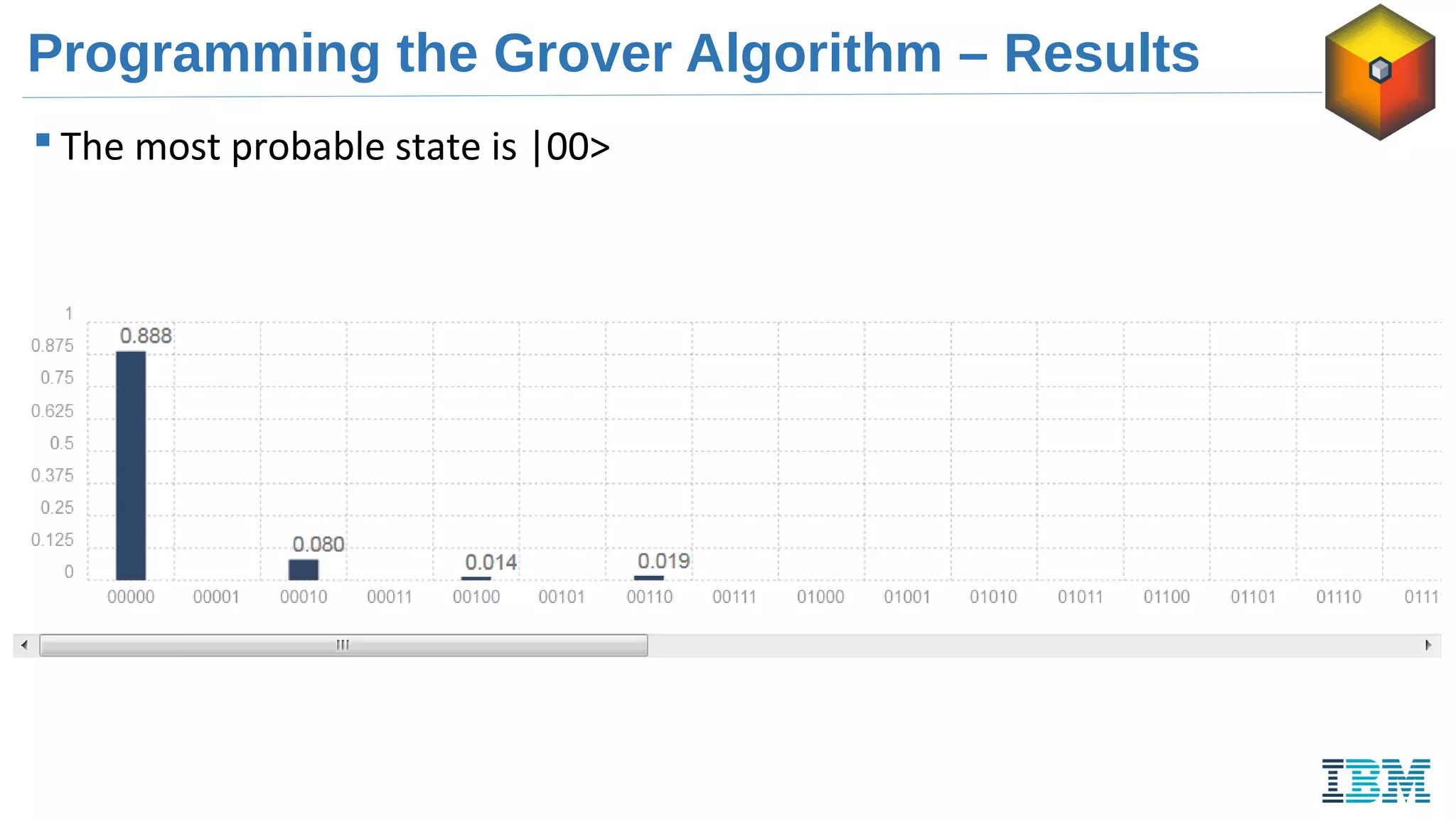
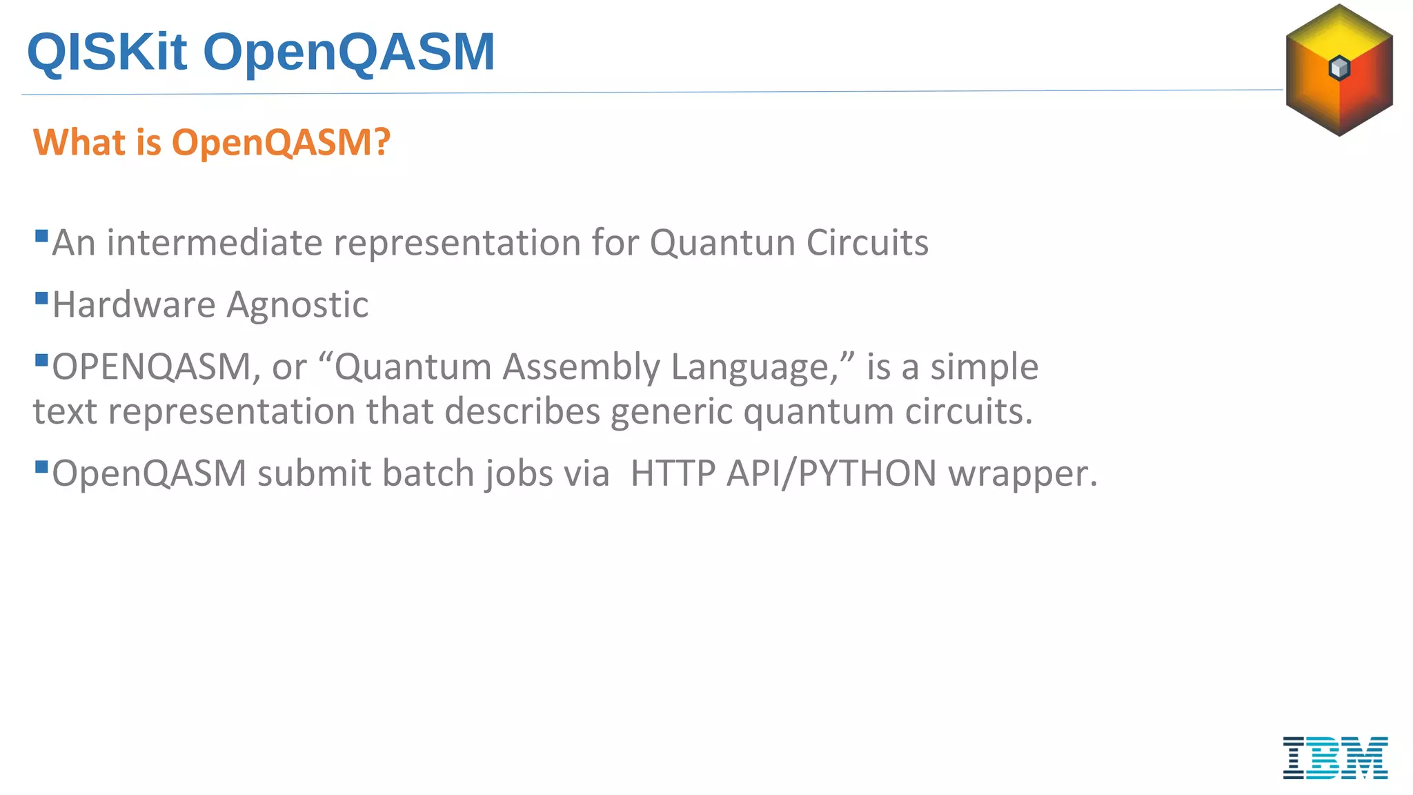
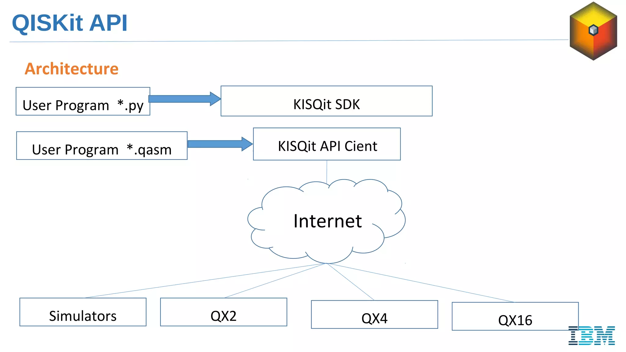
Descripcion about IBM quantum experience. In this presentation I introduce the IBM Tools for quantum programming. Also it serves as a general introduction to Quantum Computing
Labelling Requirements and Label Claims for Dietary Supplements and Recommend...
2017 10 17_quantum_program_v2
1. Quantum Programming
A New Approach to Solve Complex Problems
Francisco Gálvez Ramirez
IBM Staff
fjgramirez@es.ibm.com
2. Introducing myself
Francisco Gálvez
BS in Experimental Physics (UV)
Master in Advanced Physics (UV)
Cloud and Integrated Systems Expert
fjgramirez@es.ibm.com
@fjgramirez
Francisco J. Galvez Ramirez
3. Agenda
Why Quantum Computation
The IBM Quantum Computer
Quantum Algorithms
How to Program a Quantum Computer
Tools for Quantum Computing
5. Why Quantum Computation ?
“...nature isn't classical, dammit, and if you want to make a simulation
of nature, you'd better make it quantum mechanical...” –
Richard Feynman, Simulating Physics with Computers
6. Why Quantum Computation ?
A qubit is the quantum concept of a bit.
0 1 It’s not any element or device. It’s a logical concept
that can be implemented on a wide range of
different systems with quantum behaviour
As a bit, a single qubit can represent two states 0
and 1
But additionally a qubit is able to manage all possible combinations
amont base states 0 and 1
10 βα +
10 βαψ +=
What is a Qubit?
7. Why Quantum Computation ?
Spin Qubits – Electron or nuclear spins on a solid Substract.
Superconducting Circuits – currents superposition around a superconductor.
Ion’s Traps– Trap ions in electric fields
Photonic Circuits – The qubits are photons driven in in silicon circuits.
Qubit Implementation
8. Why Quantum Computation ?
2 BITS
0
1
0 0
0
1
0
1
A 0 0 + B 1 0 + C 0 1 + D 1 1
1 0
0 1
1 1
2 QUBITS
One state made of a combination
of every possible state of the
system
Quantum Superposition
9. Why Quantum Computation ?
Quantum Entanglement
1. Preparing an
entangled states.
An entangled stated can be
prepared by applying a common
operation to the system.
2. Measurement
0
1
11. March - 2016: Quantum Computing in the
Cloud
IBM scientists have built a quantum processor
that any user can access through the first
quantum computing platform available in the
cloud.
IBM Quantum Experience, allows users to
execute algorithms and experiments on a real
quantum processor
12. Marzo-2017: IBM announces IBM Q
IBM Q is the new line of Quantum Computers
IBM announces the building of a quantum computer of 50 qubits and
that will offer services of quantum computation in the cloud
13. Mayo-2017: First Commercial Quantum
Computer
16 and 17 qubits universal quantum computers
IBM announces a prototype of
17 qubits commercial quantum
computing
IBM has discovered how to
scale quantum architecture
In three years it is planned to
reach 50 qubits
15. Coherence Times
• Coherence in IBM today is about
100 microseconds
• There are several initiatives to
improve the coherence times:
• Different materials
• Redesign of geometries
• Cavity Quality
• IR Shielding
• Important progress has been
made in the last decade
17. The Dilution Refrigerator
A key piece of the Quantum Computer is the Dilution Refrigerator
Working Temperature 15 mK
Dilution Refrigerator
3
He + 4
He
22. Shor Algorithm
• Number of steps that a classic computer needs to run in order
to find the prime factors of a number N of x digits
It grows exponencially with x
• The Shor algorithm is made up of two parts:
1. One Classical part - Which focuses on finding the period
of a function
2. A quantum part based on QFT technics
In 2001, IBM and Stanford University, executed for the first time the Shor algorithm in the first quantum computer of 7
qubits developed in Los Álamos.
https://www-03.ibm.com/press/us/en/pressrelease/965.wss
23. Grover Algorithm
• How many attempts need a data search in an unordered N-
element database to locate a particular element?
An average of N/2 attemps are needed)
http://www.dma.eui.upm.es/MatDis/Seminario4/AlgoritmoGrover.pdf
• A Quantum Computer executing the Grover Algorithm would
run attempsN
25. Quantum Circuits
The Circuit Model
Gates execution time ~ 25 ns
~25 ns~25 ns ~25 ns ... ... ... ... ...
Coherence time 100 ms
measurement
26. Quantum Operations
X-Gate
Flips a qubit from a 0 to a 1, or vice versa.
Hadamard Gate
Puts a qubit into a superposition of states.
Flips a second qubit only if the first qubit is 1.
Controlled Not Gate
Entanglement
H gate puts the first qubit in a
superposition. CNOT gate both
flips and does not flip the
second qubit.
Assuming the qubits start as 0,
when measured, they will be 11
or 00, but never 10 or 01.
27. Quantum Operations
It is a basic circuit that acts on one or several qubits
It is equivalent to logical gates in digital circuits
Quantum Gates
1. Quantum Gates are Reversible
2. Matematically are represented by unitary matrices.
3. The qubits upon they act keep their quantum nature.
−
=
11
11
2
1
=
0100
1000
0010
0001
=
Hadamard Gate
C-NOT Gate
=
01
10
X - Gate
28. NOT Gate
Transforms the state in
the state and viceversa
It means a rotation of π
radians around X axis
0
1
Change of state
One Qubit Quantum Gates
29. One Qubit Quantum Gates
Hadamard Gate
It transforms any of the base
states or in a
combination of both
It means a rotation of π/2
radians around X axis and Z
axis
Superposition of base states
0 1
It cannot be meassured on Z axis, but we can use an H gate to change the basis
30. One Qubit Quantum Gates
The Z Gate Cambio de Fase - π
It runs a rotation of π radians
around Z axis
31. One Qubit Quantum Gates
The S Gate Phase Shift: – π/2
It run a rotation of π/2
radians around Z axis
32. One Qubit Quantum Gates
The S Gate
Phase Shift: – π/4
It runs a rotation of π/4
radians around Z axis
33. Two Qubit Quantum Gates
The CNOT Gate
Flips the target qubit, depending on the state
of the control qubit
34. Gates with more than two qubits
The Toffoli Gate
Flips the target qubit, depending on the state
of two control qubits
control 1
control 2
target
38. Quantum Operations
The Bloch Sphere
Standard Basis is not enough to specify a quantum State.
We need to specify a phase as well.
Bloch Sphere depicts the amplitudes and the phase of
one state.
1
2
0
2
cos
+
=
θθ
ψ φ
senei
There’s a one-to-one correspondence between pure qubits
states and the points on the surface on a unit sphere
2
C 3
R
39. Quantum Operations
The Qsphere
Qsphere shows states of more than 1 qubit
For 1 qubit 2 points
For 2 qubit 3 points
for n qubit (n+1) points
Each line from the center is possible outcome
Allows to distinguish classical states from entangled states
• A classical state will have a single line pointing in one direction
• A superposition of two basis states will have two lines pointing in two directions of half
weight.
41. Tools for Quantum Programming
IBM Quantum Experience
Visual interface, Drag and Drop for 5 qubits
QISKit OpenQASM
Asembler Language for representing Quantum
Circuits
QISKit API
Python API to create and execute Quantum Circuits
46. Creating Scores
Graphical Interface used to create programs for the quantum processor
It allows to create quantum circuits using a logical gates library and well defined points of
measurement
47. Running Scores
Bar Chart
• 0’s & 1’s combination in the bottom means the measured Qubit state.
• The height of the bar represents how often that particular state occurs
48. Tools For Quantum Programming
IBM Quantum Experience QX2, QX4
Grover Algorithm
49. 1 2 3 4 ... ... N=2nω
Programming the Grover Algorithm – (I)
A list of N item and there’s one item with a unique property that we wish to locate
A classical computation needs to check on average of this boxes2N
On a quantum computer, using the Grover’s algorithm it can be done in aprox. stepsN
1 2 3 4
Lets do it for N = 4
50. Programming the Grover Algorithm – (II)
∑
−
=
=
1
0
1 N
x
x
N
s
At the beginning we have a uniform superposition
amplitu
de
0ψ
N
1
Items1 2 3 4
00 01 10 11
51. Programming the Grover Algorithm – (III)
We need a function such that: for the marked state:1)( =xf ω
In that way we build the “oracle” matrix: fU
( ) xxU xf
f
)(
1−=
Applying the oracle reflection: If is an unmarked item, the oracle does nothing, otherwise:x
ωω −=fU
amplitu
de
0ψ
N
1
Items
1 2 3 4
00 01 10 11
52. Programming the Grover Algorithm – (III)
We need a function such that: for the marked state:1)( =xf ω
Rotates 90º (on the basis )
Superposition Changes to the basis
Superposition Back to the basis only qubit #2
Change state of qubit #2 (based on #1)
−+ ,
−+ ,
1,0
53. Programming the Grover Algorithm – (III)
We need a function such that: for the marked state:1)( =xf ω
Superposition qubit # 2 back to the basis
Rotates 90º (on the basis )
−+ ,
−+ ,
54. Programming the Grover Algorithm
We now apply an additional reflection about the state .
In the bra-ket notation this reflection is written as:
This transformation maps the state to:
and completes the transformation:
s
12 −= ssUs
'tsU ψ
tfst UU ψψ =+1
sU
amplitu
de
0ψ
Items
1 2 3 4
00 01 10 11
64. QISKit OpenQASM
What is OpenQASM?
An intermediate representation for Quantun Circuits
Hardware Agnostic
OPENQASM, or “Quantum Assembly Language,” is a simple
text representation that describes generic quantum circuits.
OpenQASM submit batch jobs via HTTP API/PYTHON wrapper.
67. QISKit OpenQASM
Predefined Gates
// These are the predefined gates
U(theta,phi,lambda) qubit|qreg;
CX qubit|qreg,qubit|qreg;
New Gate Definition
// This is the definition
gate name(params) qargs
{
body
}
// This is an example
gate g a
{
U(0,0,0) a;
}
gate crz(theta) a,b
{
U(0,0,theta/2) a;
CX a,b;
U(0,0,-theta/2) b;
CX a,b;
U(0,0,theta/2) b;
}
crz(pi/2) q[0],q[1];
68. QISKit OpenQASM
Example: Quantum Fourier Transform// quantum Fourier
transform
IBMQASM 2.0;
include "qelib1.inc";
qreg q[4];
creg c[4];
x q[0];
x q[2];
barrier q;
h q[0];
cu1(pi/2) q[1],q[0];
h q[1];
cu1(pi/4) q[2],q[0];
cu1(pi/2) q[2],q[1];
h q[2];
cu1(pi/8) q[3],q[0];
cu1(pi/4) q[3],q[1];
cu1(pi/2) q[3],q[2];
h q[3];
measure q -> c;
The quantum Fourier transform demonstrates parameter
passing to gate subroutines.
This circuit applies the QFT to the state
and measures in the computational basis.
=3210 qqqq 0101
70. QISKit API
What is QISKit API?
Access to IBM’s Quantum Experience using a Python interface.
This interface allows working with quantum circuits and executing multiple
circuits in an efficient batch of experiments.
To try this out for yourself, go into the Composer and create a new experiment with three qubits. Drag a pink measurement gate over to each of them and click “Run” or “Simulate.” At this point, there should be only one possible outcome, 000. That’s because all of the qubits began in the state and we haven’t changed them with any gates. Now, drag a blue H gate to each of the qubits before the measurement. The H gate puts each of the qubits into an equal superposition state. Now you should see that there are many more possible outcomes. We’ll go into more detail about the H gate in a later section.
IBMQASM 2.0; Denotes a le in IBM QASM formata IBMQASM 2.0;
qreg name[size]; Declare a named register of qubits qreg q[5];
creg name[size]; Declare a named register of bits creg c[5];
include "filename"; Open and parse another source le include "qelib1.inc";
gate name(params) qargs { body } Declare a unitary gate (see text)
opaque name(params) qargs; Declare an opaque gate (see text)
// comment text Comment a line of text // oops!
U(theta,phi,lambda) qubit|qreg; Apply built-in single qubit gate(s)b U(pi/2,2*pi/3,0) q[0];
CX qubit|qreg,qubit|qreg; Apply built-in CNOT gate(s) CX q[0],q[1];
measure qubit|qreg -> bit|creg; Make measurement(s) in Z basis measure q -> c;
reset qubit|qreg; Prepare qubit(s) in j0i reset q[0];
gatename(params) qargs; Apply a user-dened unitary gate crz(pi/2) q[1],q[0];
if(creg==int) qop; Conditionally apply quantum operation if(c==5) CX q[0],q[1];
barrier qargs; Prevent transformations across this source line