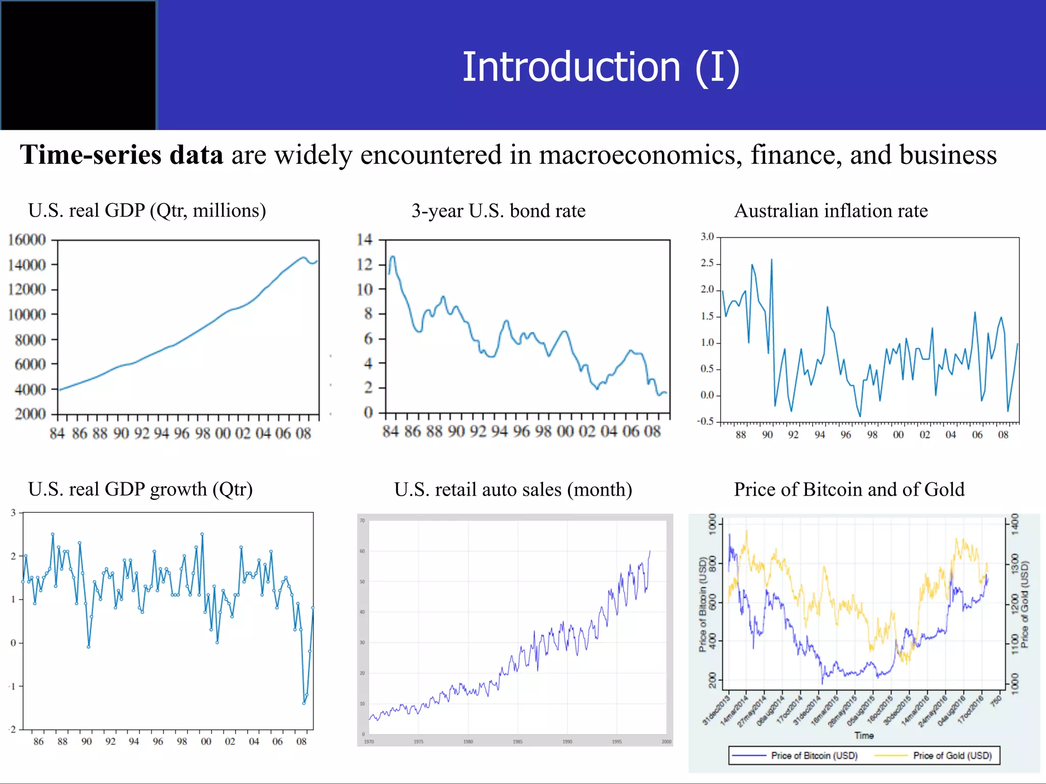
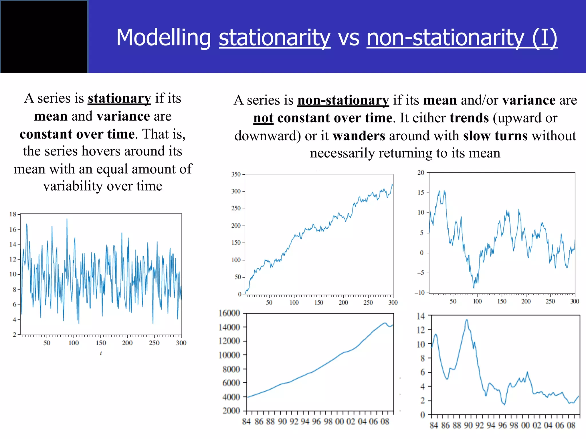
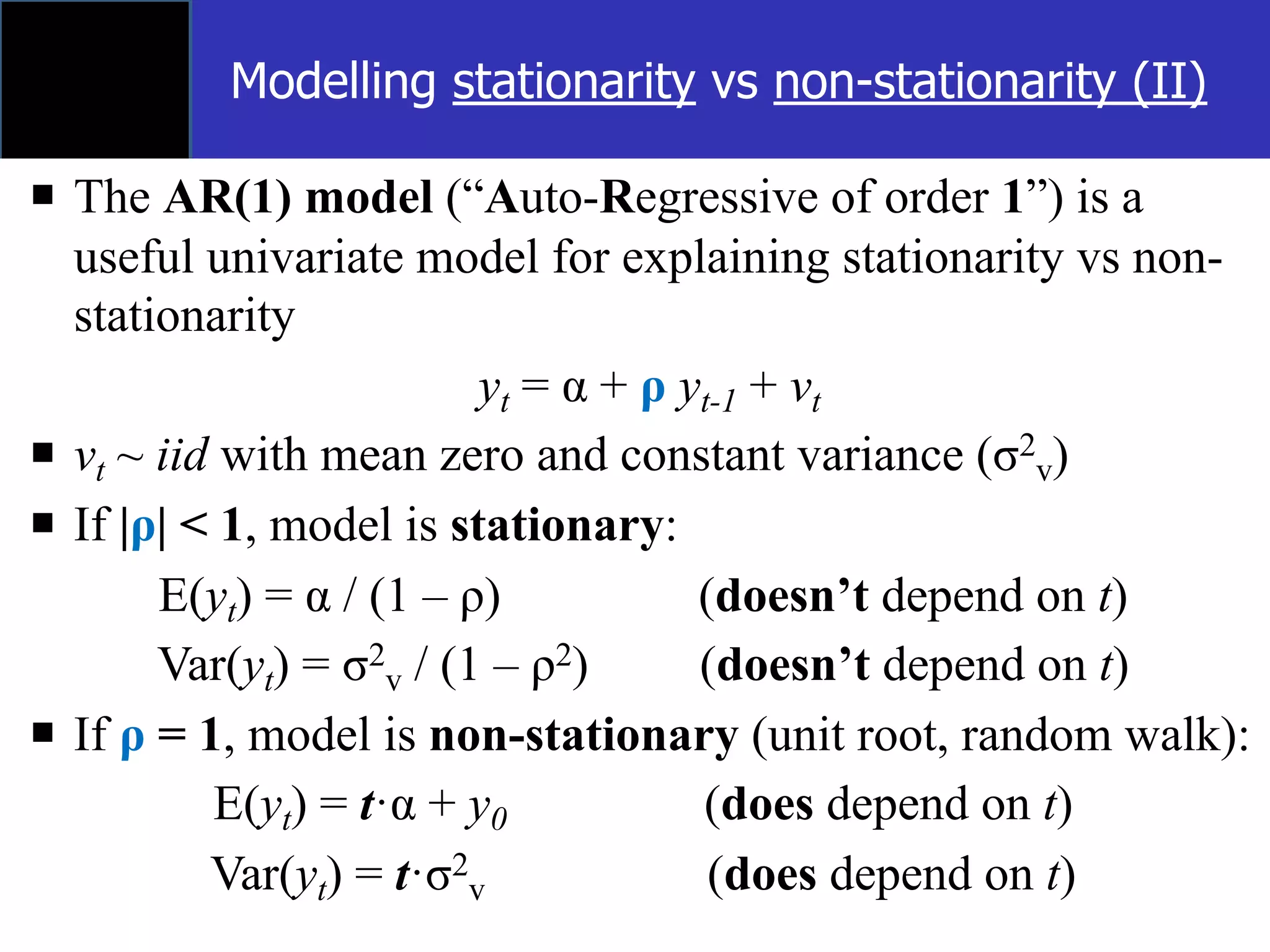
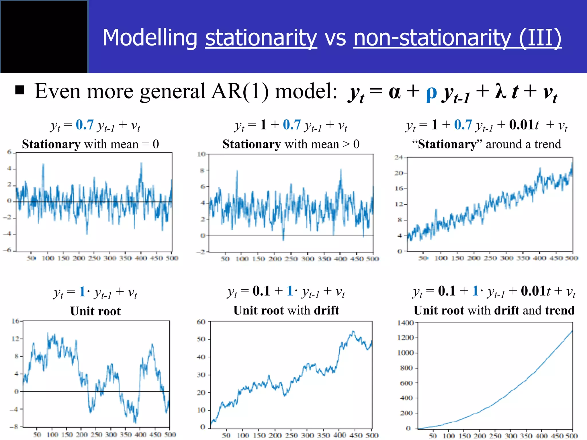
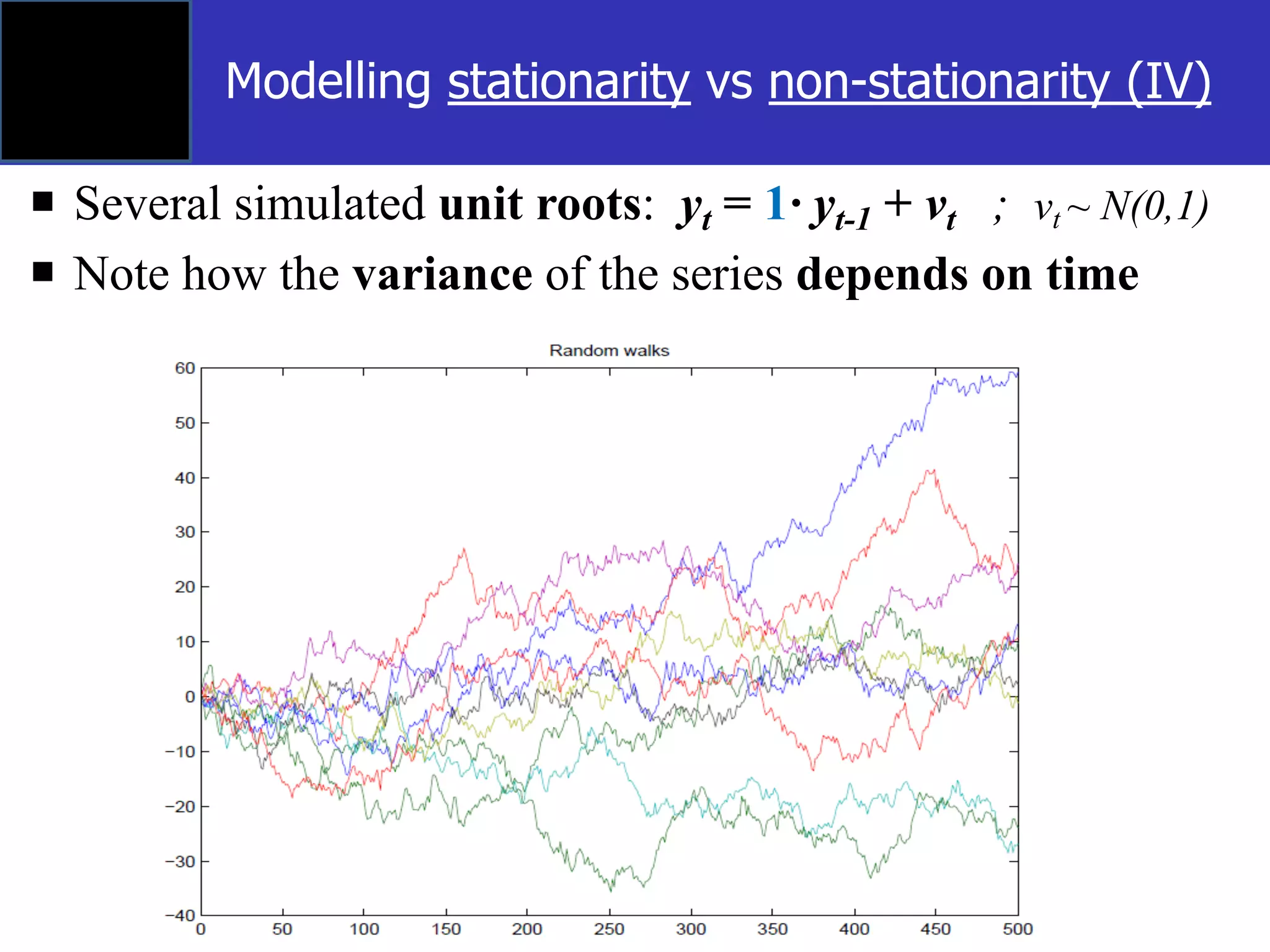
Innovations in technology has revolutionized financial services to an extent that large financial institutions like Goldman Sachs are claiming to be technology companies! It is no secret that technological innovations like Data science and AI are changing fundamentally how financial products are created, tested and delivered. While it is exciting to learn about technologies themselves, there is very little guidance available to companies and financial professionals should retool and gear themselves towards the upcoming revolution. In this master class, we will discuss key innovations in Data Science and AI and connect applications of these novel fields in forecasting and optimization. Through case studies and examples, we will demonstrate why now is the time you should invest to learn about the topics that will reshape the financial services industry of the future! Topics in Econometrics

1. Some basics of time-series
and forecasting
2019 Copyright QuantUniversity LLC.
Presented By:
Gustavo Vicentini,PhD
QuantUniversity
Econometrics Lead

2. • Gustavo leads Econometrics and Forecasting
programs at QuantUniversity.
• Gustavo worked several years as an economist at
Analysis Group and currently serves as
an associate teaching professor in the Department
of Economics at Northeastern University.
• Gustavo received a PhD in economics from Boston
University.
Gustavo Vicentini, PhD
Econometrics Lead
2

3. Principles of Econometrics, 4th Edition Page 3
Chapter 9: Regression with Time Series Data:
Stationary Variables
Some basics of time-series
and forecasting
Gustavo Vicentini
Quant University – Econometrics Lead

4. Principles of Econometrics, 4th Edition Page 4
Chapter 9: Regression with Time Series Data:
Stationary Variables
Introduction (I)
U.S. real GDP growth (Qtr)
Time-series data are widely encountered in macroeconomics, finance, and business
U.S. real GDP (Qtr, millions) 3-year U.S. bond rate Australian inflation rate
U.S. retail auto sales (month) Price of Bitcoin and of Gold

5. Principles of Econometrics, 4th Edition Page 5
Chapter 9: Regression with Time Series Data:
Stationary Variables
¡ Time-series Econometrics is very useful to analyze time-
series data
¡ Policy analysis
¡ Quantification of monetary policy: If Fed lowers
interest rate this quarter, how is current and future
GDP growth affected?
¡ Forecasting
¡ Using past data on inflation, what is a good
forecast for future inflation?
¡ Before using regression on time-series data, one needs to
test whether the series are stationary or non-stationary
¡ Why? Non-stationary series can give spurious
regression results if not handled properly
Introduction (II)

6. Principles of Econometrics, 4th Edition Page 6
Chapter 9: Regression with Time Series Data:
Stationary Variables
Modelling stationarity vs non-stationarity (I)
A series is non-stationary if its mean and/or variance are
not constant over time. It either trends (upward or
downward) or it wanders around with slow turns without
necessarily returning to its mean
A series is stationary if its
mean and variance are
constant over time. That is,
the series hovers around its
mean with an equal amount of
variability over time

7. Principles of Econometrics, 4th Edition Page 7
Chapter 9: Regression with Time Series Data:
Stationary Variables
¡ The AR(1) model (“Auto-Regressive of order 1”) is a
useful univariate model for explaining stationarity vs non-
stationarity
yt = α + ρ yt-1 + vt
¡ vt ~ iid with mean zero and constant variance (σ2
v)
¡ If |ρ| < 1, model is stationary:
E(yt) = α / (1 – ρ) (doesn’t depend on t)
Var(yt) = σ2
v / (1 – ρ2) (doesn’t depend on t)
¡ If ρ = 1, model is non-stationary (unit root, random walk):
E(yt) = t·α + y0 (does depend on t)
Var(yt) = t·σ2
v (does depend on t)
Modelling stationarity vs non-stationarity (II)

8. Principles of Econometrics, 4th Edition Page 8
Chapter 9: Regression with Time Series Data:
Stationary Variables
¡ Even more general AR(1) model: yt = α + ρ yt-1 + λ t + vt
Modelling stationarity vs non-stationarity (III)
yt = 0.7 yt-1 + vt yt = 1 + 0.7 yt-1 + vt yt = 1 + 0.7 yt-1 + 0.01t + vt
Unit root
Stationary with mean > 0 “Stationary” around a trend
yt = 1· yt-1 + vt
Stationary with mean = 0
yt = 0.1 + 1· yt-1 + vt
Unit root with drift
yt = 0.1 + 1· yt-1 + 0.01t + vt
Unit root with drift and trend

9. Principles of Econometrics, 4th Edition Page 9
Chapter 9: Regression with Time Series Data:
Stationary Variables
¡ Several simulated unit roots: yt = 1· yt-1 + vt ; vt ~ N(0,1)
¡ Note how the variance of the series depends on time
Modelling stationarity vs non-stationarity (IV)

10. Principles of Econometrics, 4th Edition Page 10
Chapter 9: Regression with Time Series Data:
Stationary Variables
¡ To test whether a series is stationary or non-stationary
one needs to test whether:
ρ = 1 (non-stationary) vs ρ < 1 (stationary)
¡ This is the Dickey-Fuller test
¡ If non-stationary (ρ = 1), then convert to its stationary
version before analyzing it. Otherwise spurious regression
¡ If series already stationary (ρ < 1), then it’s ready for
regression
¡ For the time being, let’s assume your data are stationary
and “ready” for policy analysis and forecasting
¡ (We’ll return to Dickey-Fuller later)
Modelling stationarity vs non-stationarity (V)

11. Principles of Econometrics, 4th Edition Page 11
Chapter 9: Regression with Time Series Data:
Stationary Variables
An example of policy analysis:
Monetary policy
Quarterly data on GDP growth (“y” variable) and interest rate (“x”)
How does a change in interest rate now affects GDP growth over time
(i.e., monetary policy)?
Regress y on “q” lagged values of x
yt = β0 + β1 xt-1 + β2 xt-2 + … + βq xt-q + vt
β1 is the one-quarter-ahead effect, β2 is the two-quarters-ahead
effect, and so on
If both y and x stationary, then use OLS regression to estimate the
β’s. This provides a quantification of monetary policy
A lag selection criterion should be used to select “q”
– Popular ones are AIC and BIC (similar to R2)
Can also include “quarter dummies” to control for seasonality
Can also use lagged values of yt to improve fit

12. Principles of Econometrics, 4th Edition Page 12
Chapter 9: Regression with Time Series Data:
Stationary Variables
An application of policy analysis:
Okun’s Law (I)
Okun’s Law: “U” = unemployment rate; “G” = GDP growth
Change in unemployment depends on how growth deviates from
“normal” growth rate “GN”
Its “econometric” version:
Lags of growth can be included:
If both “DU” and “G” series are stationary, then OLS
regression can be used to estimate the β’s
( )1t t t NU U G Gg-- = - -
0βt t tDU G ea= + +
0 1 1 2 2β β β βt t t t q t q tDU G G G G ea - - -= + + + + + +!

13. Principles of Econometrics, 4th Edition Page 13
Chapter 9: Regression with Time Series Data:
Stationary Variables
An application of policy analysis:
Okun’s Law (II)
§ Quarterly U.S. data:
“DU ” “G ”

14. Principles of Econometrics, 4th Edition Page 14
Chapter 9: Regression with Time Series Data:
Stationary Variables
An application of policy analysis:
Okun’s Law (III)
§ OLS regression results:
§ Recall: Number of lags can be selected with AIC or BIC

15. Principles of Econometrics, 4th Edition Page 15
Chapter 9: Regression with Time Series Data:
Stationary Variables
An example of forecasting:
Monetary policy
After estimating the β’s, then forecast future growth. A
one-quarter-ahead (“T+1”) forecast is ŷT+1:
ŷT+1 = β̂0 + β̂1 xT + β̂2 xT-1 + … + β̂q xT-q+1
The β̂ ’s are the OLS estimates
Then calculate a standard error (S.E.) for the forecast ŷT+1,
and use it to construct a 95% confidence interval for ŷT+1:
95% C.I. for ŷT+1 = ( ŷT+1 – 1.96·SE , ŷT+1 + 1.96·SE )
Could also calculate a two-quarters-ahead forecast and
confidence interval, and so on

16. Principles of Econometrics, 4th Edition Page 16
Chapter 9: Regression with Time Series Data:
Stationary Variables
An application of forecasting:
Future growth based on past growth (I)
Consider an AR(2) model for real GDP growth:
Gt = β0 + β1 Gt-1 + β2 Gt-2 + vt
Using data from 1986Q1 to 2009Q3, OLS estimates yield:
β̂0 = 0.467 β̂1 = 0.377 β̂2 = 0.246
Given that:
GT = G2009Q3 = 0.8% and GT-1 = G2009Q2 = -0.2%,
The one-quarter-ahead forecast is:
Ĝ2009Q4 = ĜT+1 = β̂0 + β̂1 GT + β̂2 GT-1
Ĝ2009Q4 = ĜT+1 = 0.718%

17. Principles of Econometrics, 4th Edition Page 17
Chapter 9: Regression with Time Series Data:
Stationary Variables
An application of forecasting:
Future growth based on past growth (II)
The two-quarters-ahead forecast is:
Ĝ2010Q1 = ĜT+2 = β̂0 + β̂1 ĜT+1 + β̂2 GT = 0.933%
And so on into further quarters…
After computing the standard errors, we can tabulate the
forecasts and confidence intervals:

18. Principles of Econometrics, 4th Edition Page 18
Chapter 9: Regression with Time Series Data:
Stationary Variables
Many economic/finance data are non-stationary (unit root):
If series is non-stationary, it shouldn’t be used (in its “raw” form) in a
regression, because OLS estimator will not behave well
Need to transform into a stationary series and then use that in the
regression
The transformation is just its first-difference: Dyt = yt – yt-1
For example, if both y and x are non-stationary, you should
Use: Dyt = β0 + β1 Dxt + ut And not use: yt = β0 + β1 xt + ut
Handling non-stationary series (I)
3-year U.S. bond rate Bitcoin price U.S. inflation rate

19. Principles of Econometrics, 4th Edition Page 19
Chapter 9: Regression with Time Series Data:
Stationary Variables
Examples of the first-difference transformation:
Handling non-stationary series (II)

20. Principles of Econometrics, 4th Edition Page 20
Chapter 9: Regression with Time Series Data:
Stationary Variables
§ Why can’t use “raw” version of non-stationary series in a regression?
Because the potential of “spurious regression”
§ Consider two unit roots that were independently simulated (they are not
related to each other)
§ An OLS regression of rw1 on rw2 yields:
§ These results are statistically significant (t = 40.8 and R2 = 0.70!!), but
completely meaningless, or spurious. The apparent significance is false
Handling non-stationary series (III)
2
1 217.818 0.842 , 0.70
( ) (40.837)
t trw rw R
t
= + =

21. Principles of Econometrics, 4th Edition Page 21
Chapter 9: Regression with Time Series Data:
Stationary Variables
First thing is to test whether the series is non-stationary
If series is stationary, then work with the series itself
(without taking first-difference)
If series is non-stationary, then work with first-difference
Dickey-Fuller (“DF”) test used to test non-stationarity
Consider again the AR(1) model:
A more convenient form is:
Run this last regression, and test whether γ = 0 or γ < 0
Handling non-stationary series (IV)
1t t ty y v-= r +
( )
1 1 1
1
1
1
t t t t t
t t t
t t
y y y y v
y y v
y v
- - -
-
-
- = r - +
D = r - +
= g +

22. Principles of Econometrics, 4th Edition Page 22
Chapter 9: Regression with Time Series Data:
Stationary Variables
Dickey-Fuller critical values for γ̂
If γ̂ is less then the critical value(s), we reject the
hypothesis of non-stationarity
Handling non-stationary series (V)
1t t ty y v-= r + ( )
1 1 1
1
1
1
t t t t t
t t t
t t
y y y y v
y y v
y v
- - -
-
-
- = r - +
D = r - +
= g +

References:

1- https://www.h2o.ai/resources/white-paper/machine-learning-considerations-for-fairly-and-transparently-expanding-access-to-credit/
2- https://arxiv.org/abs/2011.03156
Seeing what a gan cannot generate: paper reviewQuantUniversity
Seeing what a GAN cannot Generate Paper review: Bau, David et al. “Seeing What a GAN Cannot Generate.” 2019 IEEE/CVF International Conference on Computer Vision (ICCV) (2019): 4501-4510.
Machine Learning in Finance: 10 Things You Need to Know in 2021QuantUniversity
Machine Learning and AI has revolutionized Finance! In the last five years, innovations in computing, technology and business models have created multiple products and services in Fintech prompting organizations to prioritize their data and AI strategies. What will 2021 bring and how should you prepare for it? Join Sri Krishnamurthy,CFA as we kickoff the QuantUniversity’s Winter school 2021. We will introduce you to the upcoming programs and have a masterclass on 10 innovations in AI and ML you need to know in 2021!
Markowitz portfolio optimization is optimal in theory, however, when applied in practice it often fails catastrophically. Usually, this is addressed by various simplifications to increase robustness. In this talk I will make the case that the reason this theory fails in practice is because uncertainty in the parameter estimation is not taken into account. By using Bayesian statistics we can fix Markowitz and retain all its desirable properties while still having a robustness technique that can be easily extended. This talk is geared at intermediate and will give a general introduction to Bayesian modeling using PyMC3 and focus on application and code examples rather than theory.
With Alternative Data becoming more and more popular in the industry, quants are eager to adopt them into their investment processes. However, with a plethora of options, API standards, trying and evaluating datasets is a major hindrance to adoption of datasets.
Join Yaacov, Sri, James and Brad discuss the opportunities, pitfalls and challenges of Alternative Data and its adoption in finance
A Unified Framework for Model Explanation
Ian Covert, University of Washington
Explainable AI is becoming increasingly important, but the field is evolving rapidly and requires better organizing principles to remain manageable for researchers and practitioners. In this talk, Ian will discuss a new paper that unifies a large portion of the literature using a simple idea: simulating feature removal. The new class of "removal-based explanations" describes 20+ existing methods (e.g., LIME, SHAP) and reveals underlying links with psychology, game theory and information theory.
Practical examples will be presented and available on the Qu.Academy site
Reference:
Explaining by Removing: A Unified Framework for Model Explanation
Ian Covert, Scott Lundberg, Su-In Lee
https://arxiv.org/abs/2011.14878
Machine Learning Interpretability -
Self-Explanatory Models: Interpretability, Diagnostics and Simplification
With Agus Sudjianto, Wells Fargo
The deep neural networks (DNNs) have achieved great success in learning complex patterns with strong predictive power, but they are often thought of as "black box"models without a sufficient level of transparency and interpretability. It is important to demystify the DNNs with rigorous mathematics and practical tools, especially when they are used for mission-critical applications. This talk aims to unwrap the black box of deep ReLU networks through exact local linear representation, which utilizes the activation pattern and disentangles the complex network into an equivalent set of local linear models (LLMs). We develop a convenient LLM-based toolkit for interpretability, diagnostics, and simplification of a pre-trained deep ReLU network. We propose the local linear profile plot and other visualization methods for interpretation and diagnostics, and an effective merging strategy for network simplification. The proposed methods are demonstrated by simulation examples, benchmark datasets, and a real case study in credit risk assessment. The paper that will be presented in this talk can be found here.
Qu speaker series 14: Synthetic Data Generation in FinanceQuantUniversity
In this master class, Stefan shows how to create synthetic time-series data using generative adversarial networks (GAN). GANs train a generator and a discriminator network in a competitive setting so that the generator learns to produce samples that the discriminator cannot distinguish from a given class of training data. The goal is to yield a generative model capable of producing synthetic samples representative of this class. While most popular with image data, GANs have also been used to generate synthetic time-series data in the medical domain. Subsequent experiments with financial data explored whether GANs can produce alternative price trajectories useful for ML training or strategy backtests.
In 2009 author and motivational speaker Simon Sinek delivered the now-classic TED talk “Start with why”. Viewed by over 28 million people, “Start with Why” is the third most popular TED video of all time and it teaches us that great leaders and companies inspire us to take action by focusing on the WHY over the “what” or the “how”. In this talk we’ll ask how applied data and computational scientists can use the power of WHY to frame problems, inspire others, and give them answers to business questions they might never think of asking.
Bio
Jessica Stauth is a Managing Director in Fidelity Labs, an internal startup incubator with a mission to create new fintech businesses that drive growth for the firm. Dr. Stauth previously held roles as Managing Director of Portfolio Management, Research, and Trading at Quantopian, a crowd-sourced systematic hedge fund based in Boston, Director of Quant Product Strategy for Thomson Reuters (now Refinitiv), and as a Senior Quant Researcher at the StarMine Corporation, where she built global stock selection models including the design and implementation of the StarMine Short Interest model. Dr. Stauth holds a PhD in Biophysics from UC Berkeley, where her research focused on computational neuroscience.
Adjusting OpenMP PageRank : SHORT REPORT / NOTESSubhajit Sahu
For massive graphs that fit in RAM, but not in GPU memory, it is possible to take
advantage of a shared memory system with multiple CPUs, each with multiple cores, to
accelerate pagerank computation. If the NUMA architecture of the system is properly taken
into account with good vertex partitioning, the speedup can be significant. To take steps in
this direction, experiments are conducted to implement pagerank in OpenMP using two
different approaches, uniform and hybrid. The uniform approach runs all primitives required
for pagerank in OpenMP mode (with multiple threads). On the other hand, the hybrid
approach runs certain primitives in sequential mode (i.e., sumAt, multiply).
The Building Blocks of QuestDB, a Time Series Databasejavier ramirez
Talk Delivered at Valencia Codes Meetup 2024-06.
Traditionally, databases have treated timestamps just as another data type. However, when performing real-time analytics, timestamps should be first class citizens and we need rich time semantics to get the most out of our data. We also need to deal with ever growing datasets while keeping performant, which is as fun as it sounds.
It is no wonder time-series databases are now more popular than ever before. Join me in this session to learn about the internal architecture and building blocks of QuestDB, an open source time-series database designed for speed. We will also review a history of some of the changes we have gone over the past two years to deal with late and unordered data, non-blocking writes, read-replicas, or faster batch ingestion.
Adjusting primitives for graph : SHORT REPORT / NOTESSubhajit Sahu
Graph algorithms, like PageRank Compressed Sparse Row (CSR) is an adjacency-list based graph representation that is
Multiply with different modes (map)
1. Performance of sequential execution based vs OpenMP based vector multiply.
2. Comparing various launch configs for CUDA based vector multiply.
Sum with different storage types (reduce)
1. Performance of vector element sum using float vs bfloat16 as the storage type.
Sum with different modes (reduce)
1. Performance of sequential execution based vs OpenMP based vector element sum.
2. Performance of memcpy vs in-place based CUDA based vector element sum.
3. Comparing various launch configs for CUDA based vector element sum (memcpy).
4. Comparing various launch configs for CUDA based vector element sum (in-place).
Sum with in-place strategies of CUDA mode (reduce)
1. Comparing various launch configs for CUDA based vector element sum (in-place).
Unleashing the Power of Data_ Choosing a Trusted Analytics Platform.pdfEnterprise Wired
In this guide, we'll explore the key considerations and features to look for when choosing a Trusted analytics platform that meets your organization's needs and delivers actionable intelligence you can trust.
06-04-2024 - NYC Tech Week - Discussion on Vector Databases, Unstructured Data and AI
Round table discussion of vector databases, unstructured data, ai, big data, real-time, robots and Milvus.
A lively discussion with NJ Gen AI Meetup Lead, Prasad and Procure.FYI's Co-Found
Enhanced Enterprise Intelligence with your personal AI Data Copilot.pdfGetInData
Recently we have observed the rise of open-source Large Language Models (LLMs) that are community-driven or developed by the AI market leaders, such as Meta (Llama3), Databricks (DBRX) and Snowflake (Arctic). On the other hand, there is a growth in interest in specialized, carefully fine-tuned yet relatively small models that can efficiently assist programmers in day-to-day tasks. Finally, Retrieval-Augmented Generation (RAG) architectures have gained a lot of traction as the preferred approach for LLMs context and prompt augmentation for building conversational SQL data copilots, code copilots and chatbots.
In this presentation, we will show how we built upon these three concepts a robust Data Copilot that can help to democratize access to company data assets and boost performance of everyone working with data platforms.
Why do we need yet another (open-source ) Copilot?
How can we build one?
Architecture and evaluation
Enhanced Enterprise Intelligence with your personal AI Data Copilot.pdf
Econometrics