Download as PDF, PPTX
![SVM and probabilities
Some facts
SVM is universally consistent (converges towards the Bayes risk)
SVM asymptotically implements the bayes rule
but theoretically: no consistency towards conditional probabilities (due
to the nature of sparsity)
to estimate conditional probabilities on an interval
(typically[1
2 − η, 1
2 + η]) to sparseness in this interval (all data points
have to be support vectors)
Bartlett & Tewari, JMLR, 07](https://image.slidesharecdn.com/lecture8multiclasssvm-140315083056-phpapp01/85/Lecture8-multi-class_svm-12-320.jpg)
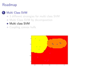
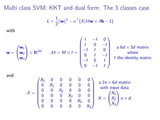
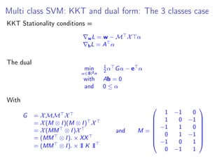
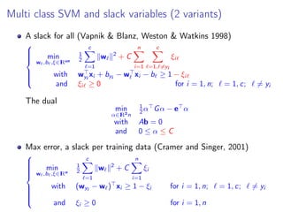
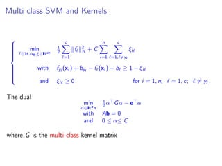
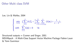
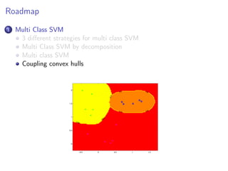
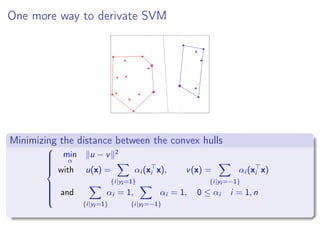
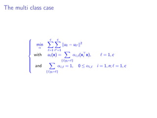

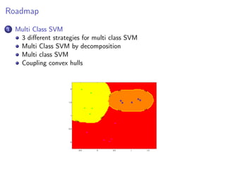
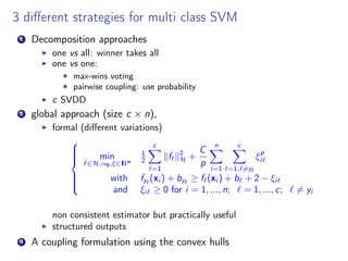
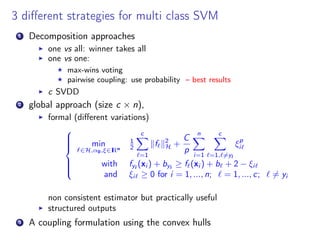
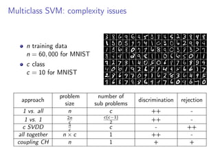
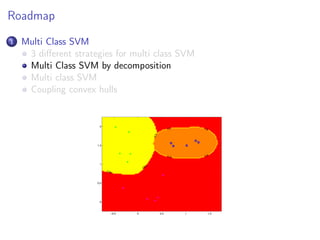
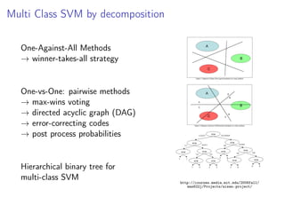
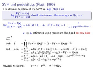
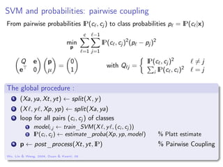
This document discusses multi-class support vector machines (SVMs). It outlines three main strategies for multi-class SVMs: decomposition approaches like one-vs-all and one-vs-one, a global approach, and an approach using pairwise coupling of convex hulls. It also discusses using SVMs to estimate class probabilities and describes two variants of multi-class SVMs that incorporate slack variables to allow misclassified examples.