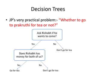
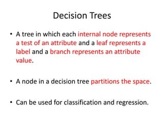
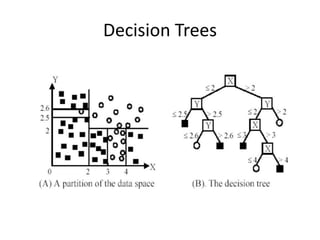
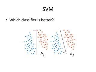
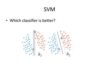
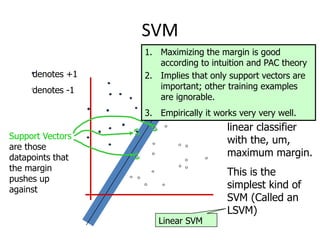
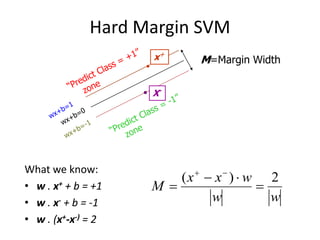
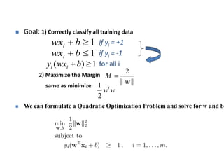
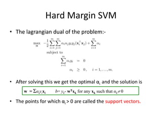
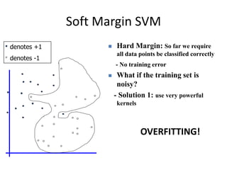
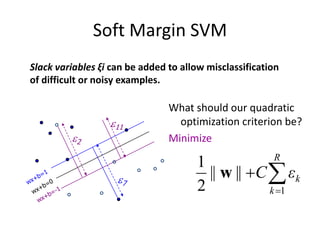
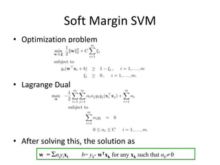
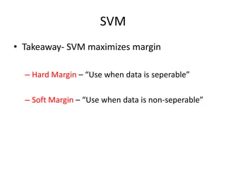
1) Decision trees are models that partition the feature space into rectangular regions and make predictions based on the region a sample falls into. They can be used for both classification and regression problems. 2) Support vector machines (SVMs) look for the optimal separating hyperplane that maximizes the margin between the classes. The hard margin SVM requires all samples to be classified correctly while the soft margin SVM allows for some misclassification using slack variables. 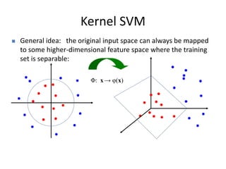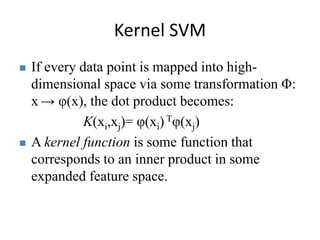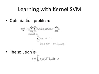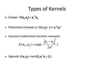3) Kernel SVMs map the input data into a higher dimensional feature space to allow for nonlinear decision boundaries using kernel functions such as the radial basis function kernel. This helps address the limitations of linear SVMs.

1. Machine Learning Interviews –
Day 2
Arpit Agarwal

2. Decision Trees
• JP’s very practical problem:- “Whether to go
to prakruthi for tea or not?”
Ask Rishabh if he
wants to come?
Yes No
Does Rishabh has
money for both of us?
Don’t go for tea
Yes No
Go for tea Don’t go for tea

3. Decision Trees
• A tree in which each internal node represents
a test of an attribute and a leaf represents a
label and a branch represents an attribute
value.
• A node in a decision tree partitions the space.
• Can be used for classification and regression.

4. Decision Trees

5. Decision Tree Learning
– Choose the best attribute to split the remaining instances
and make that attribute a decision node
– Each node will correspond to a subset of the training set
– Repeat this process recursively for each child
– Stop when:
• All the instances in a node have the same label
• There are no more attributes
• There are no more instances

6. How to select the best attribute?
• Various heuristics such as
– Entropy Impurity (which is minimized when all the
instances in a given node have same label)
• Entropy(S) = - p1 * log2(p1) - p0 * log2(p0)
– Gini Impurity
• Entropy(S) = p0 * p1

7. Decision Tree Pruning
• In pruning we remove a bad decision node
and merge its children.
• Two techniques:
– Subtree Replacement
– Subtree Raising

8. Decision Trees
• Advantage- Easy to understand and interpret;
can be applied to wide variety of problems
• Disadvantage- Difficult to learn, Overfittting
problem, Error-propagation

9. Support Vector Machine (SVM)
• Belong to the ‘Marwari’ family of algorithms
- “Always thinks about maximizing its margins”

10. SVM
• Which classifier is better?

11. SVM
• Which classifier is better?

12. SVM
denotes +1
denotes -1
f(x,w,b) = sign(w x + b)
The maximum
margin linear
classifier is the
linear classifier
with the, um,
maximum margin.
This is the
simplest kind of
SVM (Called an
LSVM)
Linear SVM
Support Vectors
are those
datapoints that
the margin
pushes up
against
1. Maximizing the margin is good
according to intuition and PAC theory
2. Implies that only support vectors are
important; other training examples
are ignorable.
3. Empirically it works very very well.

13. Hard Margin SVM
What we know:
• w . x+ + b = +1
• w . x- + b = -1
• w . (x+-x-) = 2
X-x+
M=Margin Width
x x w
w w
M
( ) 2

 

 

14.  Goal: 1) Correctly classify all training data
if yi = +1
if yi = -1
for all i
wx  b 1 i
wx  b 1 i
y (wx  b) 1 i i
2) Maximize the Margin
same as minimize
2
w
|| ||
M 
1
w w t
2
 We can formulate a Quadratic Optimization Problem and solve for w and b

15. Hard Margin SVM
• The lagrangian dual of the problem:-
• After solving this we get the optimal αi and the solution is
w = Σαiyixi b= yk- wTxk for any xk such that αk 0
• The points for which αi > 0 are called the support vectors.

16. Soft Margin SVM
 Hard Margin: So far we require
all data points be classified correctly
- No training error
 What if the training set is
noisy?
- Solution 1: use very powerful
kernels
denotes +1
denotes -1
OVERFITTING!

17. Soft Margin SVM
Slack variables ξi can be added to allow misclassification
of difficult or noisy examples.
e11
e7
e2
What should our quadratic
optimization criterion be?
Minimize


R
C εk
k
1
1
|| w
||
2

18. Soft Margin SVM
• Optimization problem
• Lagrange Dual
• After solving this, the solution as
w = Σαiyixi b= yk- wTxk for any xk such that αk 0

19. Kernel SVM
 General idea: the original input space can always be mapped
to some higher-dimensional feature space where the training
set is separable:
Φ: x → φ(x)

20. Kernel SVM
 If every data point is mapped into high-dimensional
space via some transformation Φ:
x → φ(x), the dot product becomes:
K(xi,xj)= φ(xi) Tφ(xj)
 A kernel function is some function that
corresponds to an inner product in some
expanded feature space.

21. Learning with Kernel SVM
• Optimization problem:
• The solution is

22. Types of Kernels
 Linear: K(xi,xj)= xi
Txj
 Polynomial of power p: K(xi,xj)= (1+ xi
Txj)p
 Gaussian (radial-basis function network):
i j
( , ) exp( 2
 Sigmoid: K(xi,xj)= tanh(β0xi
Txj + β1)
)
2
2

i j
x x
x x

K  

23. SVM
• Takeaway- SVM maximizes margin
– Hard Margin – “Use when data is seperable”
– Soft Margin – “Use when data is non-seperable”

24. - What is Overfitting? How to avoid it?
- “Cross-validation, regularization”
- What is regularization? Why do we need it?
- What is Bias-Variance tradeoff?

25. Overfitting – Curve Fitting

26. Overfitting