Guide

A Practical Guide to Support Vector Classification
Chih-Wei Hsu, Chih-Chung Chang, and Chih-Jen Lin
Department of Computer Science
National Taiwan University, Taipei 106, Taiwan
http://www.csie.ntu.edu.tw/~cjlin
Initial version: 2003 Last updated: April 15, 2010
Abstract
The support vector machine (SVM) is a popular classification technique.
However, beginners who are not familiar with SVM often get unsatisfactory
results since they miss some easy but significant steps. In this guide, we propose
a simple procedure which usually gives reasonable results.
1 Introduction
SVMs (Support Vector Machines) are a useful technique for data classification. Al-
though SVM is considered easier to use than Neural Networks, users not familiar with
it often get unsatisfactory results at first. Here we outline a “cookbook” approach
which usually gives reasonable results.
Note that this guide is not for SVM researchers nor do we guarantee you will
achieve the highest accuracy. Also, we do not intend to solve challenging or diffi-
cult problems. Our purpose is to give SVM novices a recipe for rapidly obtaining
acceptable results.
Although users do not need to understand the underlying theory behind SVM, we
briefly introduce the basics necessary for explaining our procedure. A classification
task usually involves separating data into training and testing sets. Each instance
in the training set contains one “target value” (i.e. the class labels) and several
“attributes” (i.e. the features or observed variables). The goal of SVM is to produce
a model (based on the training data) which predicts the target values of the test data
given only the test data attributes.
Given a training set of instance-label pairs (xi, yi), i = 1, . . . , l where xi ∈ Rn
and
y ∈ {1, −1}l
, the support vector machines (SVM) (Boser et al., 1992; Cortes and
Vapnik, 1995) require the solution of the following optimization problem:
min
w,b,ξ
1
2
wT
w + C
l
i=1
ξi
subject to yi(wT
φ(xi) + b) ≥ 1 − ξi, (1)
ξi ≥ 0.
1

Table 1: Problem characteristics and performance comparisons.
Applications #training #testing #features #classes Accuracy Accuracy
data data by users by our
procedure
Astroparticle1
3,089 4,000 4 2 75.2% 96.9%
Bioinformatics2
391 04
20 3 36% 85.2%
Vehicle3
1,243 41 21 2 4.88% 87.8%
Here training vectors xi are mapped into a higher (maybe infinite) dimensional space
by the function φ. SVM finds a linear separating hyperplane with the maximal margin
in this higher dimensional space. C > 0 is the penalty parameter of the error term.
Furthermore, K(xi, xj) ≡ φ(xi)T
φ(xj) is called the kernel function. Though new
kernels are being proposed by researchers, beginners may find in SVM books the
following four basic kernels:
• linear: K(xi, xj) = xT
i xj.
• polynomial: K(xi, xj) = (γxi
T
xj + r)d
, γ > 0.
• radial basis function (RBF): K(xi, xj) = exp(−γ xi − xj
2
), γ > 0.
• sigmoid: K(xi, xj) = tanh(γxi
T
xj + r).
Here, γ, r, and d are kernel parameters.
1.1 Real-World Examples
Table 1 presents some real-world examples. These data sets are supplied by our users
who could not obtain reasonable accuracy in the beginning. Using the procedure
illustrated in this guide, we help them to achieve better performance. Details are in
Appendix A.
These data sets are at http://www.csie.ntu.edu.tw/~cjlin/papers/guide/
data/
1
Courtesy of Jan Conrad from Uppsala University, Sweden.
2
Courtesy of Cory Spencer from Simon Fraser University, Canada (Gardy et al., 2003).
3
Courtesy of a user from Germany.
4
As there are no testing data, cross-validation instead of testing accuracy is presented here.
Details of cross-validation are in Section 3.2.
2

1.2 Proposed Procedure
Many beginners use the following procedure now:
• Transform data to the format of an SVM package
• Randomly try a few kernels and parameters
• Test
We propose that beginners try the following procedure first:
• Transform data to the format of an SVM package
• Conduct simple scaling on the data
• Consider the RBF kernel K(x, y) = e−γ x−y 2
• Use cross-validation to find the best parameter C and γ
• Use the best parameter C and γ to train the whole training set5
• Test
We discuss this procedure in detail in the following sections.
2 Data Preprocessing
2.1 Categorical Feature
SVM requires that each data instance is represented as a vector of real numbers.
Hence, if there are categorical attributes, we first have to convert them into numeric
data. We recommend using m numbers to represent an m-category attribute. Only
one of the m numbers is one, and others are zero. For example, a three-category
attribute such as {red, green, blue} can be represented as (0,0,1), (0,1,0), and (1,0,0).
Our experience indicates that if the number of values in an attribute is not too large,
this coding might be more stable than using a single number.
5
The best parameter might be affected by the size of data set but in practice the one obtained
from cross-validation is already suitable for the whole training set.
3

2.2 Scaling
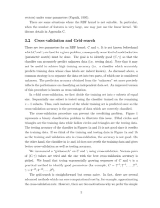
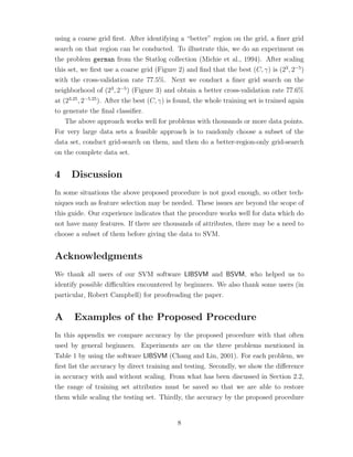
Scaling before applying SVM is very important. Part 2 of Sarle’s Neural Networks
FAQ Sarle (1997) explains the importance of this and most of considerations also ap-
ply to SVM. The main advantage of scaling is to avoid attributes in greater numeric
ranges dominating those in smaller numeric ranges. Another advantage is to avoid
numerical difficulties during the calculation. Because kernel values usually depend on
the inner products of feature vectors, e.g. the linear kernel and the polynomial ker-
nel, large attribute values might cause numerical problems. We recommend linearly
scaling each attribute to the range [−1, +1] or [0, 1].
Of course we have to use the same method to scale both training and testing
data. For example, suppose that we scaled the first attribute of training data from
[−10, +10] to [−1, +1]. If the first attribute of testing data lies in the range [−11, +8],
we must scale the testing data to [−1.1, +0.8]. See Appendix B for some real examples.
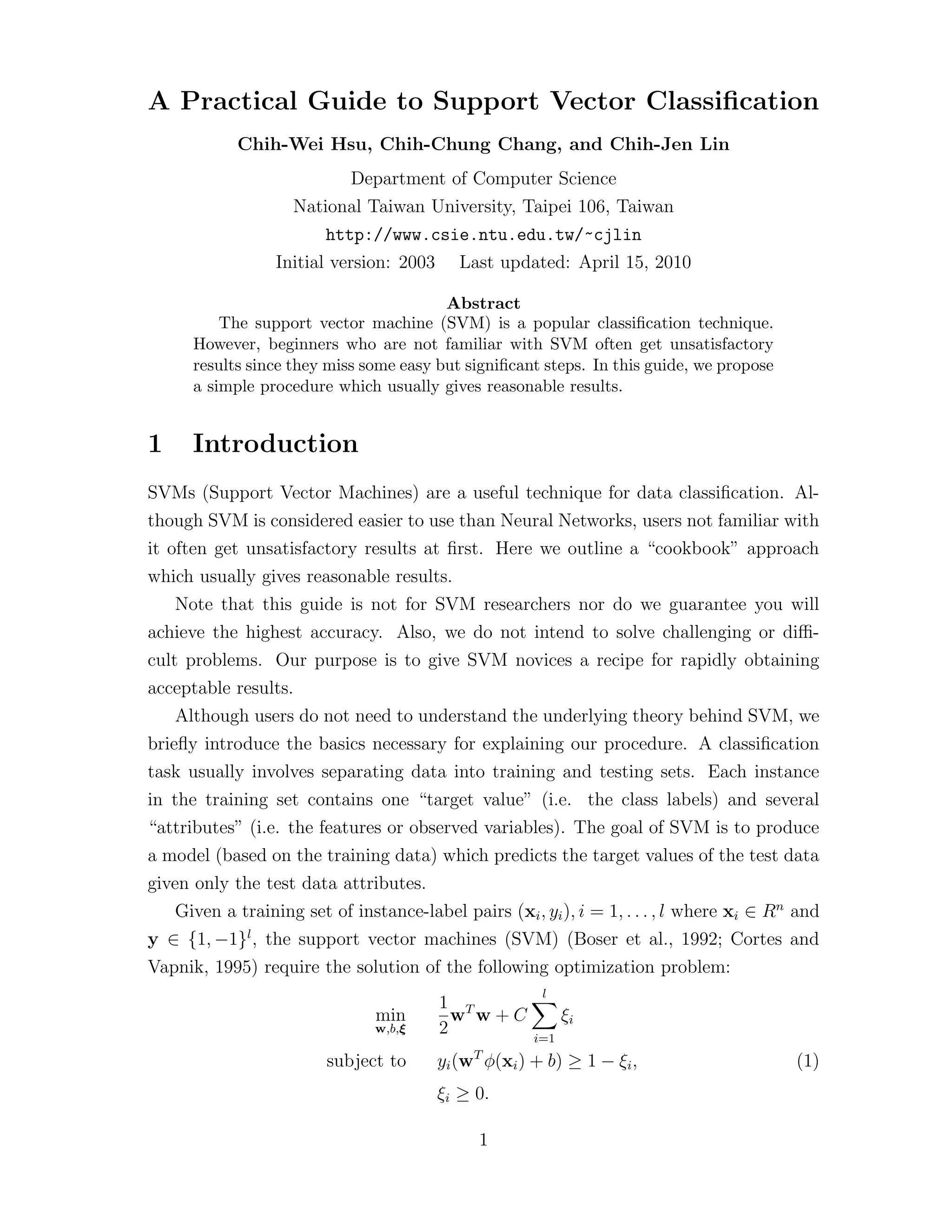
3 Model Selection
Though there are only four common kernels mentioned in Section 1, we must decide
which one to try first. Then the penalty parameter C and kernel parameters are
chosen.
3.1 RBF Kernel
In general, the RBF kernel is a reasonable first choice. This kernel nonlinearly maps
samples into a higher dimensional space so it, unlike the linear kernel, can handle the
case when the relation between class labels and attributes is nonlinear. Furthermore,
the linear kernel is a special case of RBF Keerthi and Lin (2003) since the linear
kernel with a penalty parameter ˜C has the same performance as the RBF kernel with
some parameters (C, γ). In addition, the sigmoid kernel behaves like RBF for certain
parameters (Lin and Lin, 2003).
The second reason is the number of hyperparameters which influences the com-
plexity of model selection. The polynomial kernel has more hyperparameters than
the RBF kernel.
Finally, the RBF kernel has fewer numerical difficulties. One key point is 0 <
Kij ≤ 1 in contrast to polynomial kernels of which kernel values may go to infinity
(γxi
T
xj + r > 1) or zero (γxi
T
xj + r < 1) while the degree is large. Moreover, we
must note that the sigmoid kernel is not valid (i.e. not the inner product of two
4

vectors) under some parameters (Vapnik, 1995).
There are some situations where the RBF kernel is not suitable. In particular,
when the number of features is very large, one may just use the linear kernel. We
discuss details in Appendix C.
3.2 Cross-validation and Grid-search
There are two parameters for an RBF kernel: C and γ. It is not known beforehand
which C and γ are best for a given problem; consequently some kind of model selection
(parameter search) must be done. The goal is to identify good (C, γ) so that the
classifier can accurately predict unknown data (i.e. testing data). Note that it may
not be useful to achieve high training accuracy (i.e. a classifier which accurately
predicts training data whose class labels are indeed known). As discussed above, a
common strategy is to separate the data set into two parts, of which one is considered
unknown. The prediction accuracy obtained from the “unknown” set more precisely
reflects the performance on classifying an independent data set. An improved version
of this procedure is known as cross-validation.
In v-fold cross-validation, we first divide the training set into v subsets of equal
size. Sequentially one subset is tested using the classifier trained on the remaining
v − 1 subsets. Thus, each instance of the whole training set is predicted once so the
cross-validation accuracy is the percentage of data which are correctly classified.
The cross-validation procedure can prevent the overfitting problem. Figure 1
represents a binary classification problem to illustrate this issue. Filled circles and
triangles are the training data while hollow circles and triangles are the testing data.
The testing accuracy of the classifier in Figures 1a and 1b is not good since it overfits
the training data. If we think of the training and testing data in Figure 1a and 1b
as the training and validation sets in cross-validation, the accuracy is not good. On
the other hand, the classifier in 1c and 1d does not overfit the training data and gives
better cross-validation as well as testing accuracy.
We recommend a “grid-search” on C and γ using cross-validation. Various pairs
of (C, γ) values are tried and the one with the best cross-validation accuracy is
picked. We found that trying exponentially growing sequences of C and γ is a
practical method to identify good parameters (for example, C = 2−5
, 2−3
, . . . , 215
,
γ = 2−15
, 2−13
, . . . , 23
).
The grid-search is straightforward but seems naive. In fact, there are several
advanced methods which can save computational cost by, for example, approximating
the cross-validation rate. However, there are two motivations why we prefer the simple
5

(a) Training data and an overfitting classifier (b) Applying an overfitting classifier on testing
data
(c) Training data and a better classifier (d) Applying a better classifier on testing data
Figure 1: An overfitting classifier and a better classifier (G and L: training data;
and : testing data).
grid-search approach.
One is that, psychologically, we may not feel safe to use methods which avoid
doing an exhaustive parameter search by approximations or heuristics. The other
reason is that the computational time required to find good parameters by grid-
search is not much more than that by advanced methods since there are only two
parameters. Furthermore, the grid-search can be easily parallelized because each
(C, γ) is independent. Many of advanced methods are iterative processes, e.g. walking
along a path, which can be hard to parallelize.
Since doing a complete grid-search may still be time-consuming, we recommend
6

Figure 2: Loose grid search on C = 2−5
, 2−3
, . . . , 215
and γ = 2−15
, 2−13
, . . . , 23
.
Figure 3: Fine grid-search on C = 21
, 21.25
, . . . , 25
and γ = 2−7
, 2−6.75
, . . . , 2−3
.
7

using a coarse grid first. After identifying a “better” region on the grid, a finer grid
search on that region can be conducted. To illustrate this, we do an experiment on
the problem german from the Statlog collection (Michie et al., 1994). After scaling
this set, we first use a coarse grid (Figure 2) and find that the best (C, γ) is (23
, 2−5
)
with the cross-validation rate 77.5%. Next we conduct a finer grid search on the
neighborhood of (23
, 2−5
) (Figure 3) and obtain a better cross-validation rate 77.6%
at (23.25
, 2−5.25
). After the best (C, γ) is found, the whole training set is trained again
to generate the final classifier.
The above approach works well for problems with thousands or more data points.
For very large data sets a feasible approach is to randomly choose a subset of the
data set, conduct grid-search on them, and then do a better-region-only grid-search
on the complete data set.
4 Discussion
In some situations the above proposed procedure is not good enough, so other tech-
niques such as feature selection may be needed. These issues are beyond the scope of
this guide. Our experience indicates that the procedure works well for data which do
not have many features. If there are thousands of attributes, there may be a need to
choose a subset of them before giving the data to SVM.
Acknowledgments
We thank all users of our SVM software LIBSVM and BSVM, who helped us to
identify possible difficulties encountered by beginners. We also thank some users (in
particular, Robert Campbell) for proofreading the paper.
A Examples of the Proposed Procedure
In this appendix we compare accuracy by the proposed procedure with that often
used by general beginners. Experiments are on the three problems mentioned in
Table 1 by using the software LIBSVM (Chang and Lin, 2001). For each problem, we
first list the accuracy by direct training and testing. Secondly, we show the difference
in accuracy with and without scaling. From what has been discussed in Section 2.2,
the range of training set attributes must be saved so that we are able to restore
them while scaling the testing set. Thirdly, the accuracy by the proposed procedure
8

(scaling and then model selection) is presented. Finally, we demonstrate the use
of a tool in LIBSVM which does the whole procedure automatically. Note that a
similar parameter selection tool like the grid.py presented below is available in the
R-LIBSVM interface (see the function tune).
A.1 Astroparticle Physics
• Original sets with default parameters
$ ./svm-train svmguide1
$ ./svm-predict svmguide1.t svmguide1.model svmguide1.t.predict
→ Accuracy = 66.925%
• Scaled sets with default parameters
$ ./svm-scale -l -1 -u 1 -s range1 svmguide1 > svmguide1.scale
$ ./svm-scale -r range1 svmguide1.t > svmguide1.t.scale
$ ./svm-train svmguide1.scale
$ ./svm-predict svmguide1.t.scale svmguide1.scale.model svmguide1.t.predict
• Scaled sets with parameter selection (change to the directory tools, which
contains grid.py)
$ python grid.py svmguide1.scale
· · ·
2.0 2.0 96.8922
(Best C=2.0, γ=2.0 with ﬁve-fold cross-validation rate=96.8922%)
$ ./svm-train -c 2 -g 2 svmguide1.scale
• Using an automatic script
$ python easy.py svmguide1 svmguide1.t
Scaling training data...
Cross validation...
9

Best c=2.0, g=2.0
Training...
Scaling testing data...
Testing...
Accuracy = 96.875% (3875/4000) (classification)
A.2 Bioinformatics
$ ./svm-train -v 5 svmguide2
→ Cross Validation Accuracy = 56.5217%
$ ./svm-scale -l -1 -u 1 svmguide2 > svmguide2.scale
$ ./svm-train -v 5 svmguide2.scale
• Scaled sets with parameter selection
· · ·
2.0 0.5 85.1662
(Best C=2.0, γ=0.5 with ﬁve fold cross-validation rate=85.1662%)
$ python easy.py svmguide2
Cross validation...
Best c=2.0, g=0.5
Training...
10

A.3 Vehicle
$ ./svm-train svmguide3
$ ./svm-predict svmguide3.t svmguide3.model svmguide3.t.predict
→ Accuracy = 2.43902%
$ ./svm-scale -l -1 -u 1 -s range3 svmguide3 > svmguide3.scale
$ ./svm-scale -r range3 svmguide3.t > svmguide3.t.scale
$ ./svm-train svmguide3.scale
→ Accuracy = 12.1951%
• Scaled sets with parameter selection
· · ·
128.0 0.125 84.8753
(Best C=128.0, γ=0.125 with ﬁve-fold cross-validation rate=84.8753%)
$ ./svm-train -c 128 -g 0.125 svmguide3.scale
→ Accuracy = 87.8049%
$ python easy.py svmguide3 svmguide3.t
Cross validation...
Best c=128.0, g=0.125
Training...
Scaling testing data...
Testing...
11

B Common Mistakes in Scaling Training and Test-
ing Data
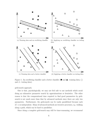
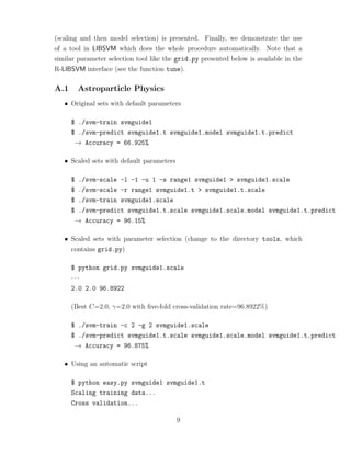
Section 2.2 stresses the importance of using the same scaling factors for training and
testing sets. We give a real example on classifying traﬃc light signals (courtesy of an
anonymous user) It is available at LIBSVM Data Sets.
If training and testing sets are separately scaled to [0, 1], the resulting accuracy is
lower than 70%.
$ ../svm-scale -l 0 svmguide4 > svmguide4.scale
$ ../svm-scale -l 0 svmguide4.t > svmguide4.t.scale
$ python easy.py svmguide4.scale svmguide4.t.scale
Using the same scaling factors for training and testing sets, we obtain much better
accuracy.
$ ../svm-scale -l 0 -s range4 svmguide4 > svmguide4.scale
$ ../svm-scale -r range4 svmguide4.t > svmguide4.t.scale
$ python easy.py svmguide4.scale svmguide4.t.scale
With the correct setting, the 10 features in svmguide4.t.scale have the following
maximal values:
0.7402, 0.4421, 0.6291, 0.8583, 0.5385, 0.7407, 0.3982, 1.0000, 0.8218, 0.9874
Clearly, the earlier way to scale the testing set to [0, 1] generates an erroneous set.
C When to Use Linear but not RBF Kernel
If the number of features is large, one may not need to map data to a higher di-
mensional space. That is, the nonlinear mapping does not improve the performance.
Using the linear kernel is good enough, and one only searches for the parameter C.
While Section 3.1 describes that RBF is at least as good as linear, the statement is
true only after searching the (C, γ) space.
Next, we split our discussion to three parts:
12

C.1 Number of instances number of features
Many microarray data in bioinformatics are of this type. We consider the Leukemia
data from the LIBSVM data sets (http://www.csie.ntu.edu.tw/~cjlin/libsvmtools/
datasets). The training and testing sets have 38 and 34 instances, respectively. The
number of features is 7,129, much larger than the number of instances. We merge the
two files and compare the cross validation accuracy of using the RBF and the linear
kernels:
• RBF kernel with parameter selection
$ cat leu leu.t > leu.combined
$ python grid.py leu.combined
· · ·
8.0 3.0517578125e-05 97.2222
(Best C=8.0, γ = 0.000030518 with five-fold cross-validation rate=97.2222%)
• Linear kernel with parameter selection
$ python grid.py -log2c -1,2,1 -log2g 1,1,1 -t 0 leu.combined
· · ·
0.5 2.0 98.6111
(Best C=0.5 with five-fold cross-validation rate=98.61111%)
Though grid.py was designed for the RBF kernel, the above way checks various
C using the linear kernel (-log2g 1,1,1 sets a dummy γ).
The cross-validation accuracy of using the linear kernel is comparable to that of using
the RBF kernel. Apparently, when the number of features is very large, one may not
need to map the data.
In addition to LIBSVM, the LIBLINEAR software mentioned below is also effective
for data in this case.
C.2 Both numbers of instances and features are large
Such data often occur in document classification. LIBSVM is not particularly good for
this type of problems. Fortunately, we have another software LIBLINEAR (Fan et al.,
2008), which is very suitable for such data. We illustrate the difference between
13

LIBSVM and LIBLINEAR using a document problem rcv1 train.binary from the
LIBSVM data sets. The numbers of instances and features are 20,242 and 47,236,
respectively.
$ time libsvm-2.85/svm-train -c 4 -t 0 -e 0.1 -m 800 -v 5 rcv1_train.binary
Cross Validation Accuracy = 96.8136%
345.569s
$ time liblinear-1.21/train -c 4 -e 0.1 -v 5 rcv1_train.binary
2.944s
For five-fold cross validation, LIBSVM takes around 350 seconds, but LIBLINEAR uses
only 3. Moreover, LIBSVM consumes more memory as we allocate some spaces to
store recently used kernel elements (see -m 800). Clearly, LIBLINEAR is much faster
than LIBSVM to obtain a model with comparable accuracy.
LIBLINEAR is efficient for large-scale document classification. Let us consider a
large set rcv1 test.binary with 677,399 instances.
$ time liblinear-1.21/train -c 0.25 -v 5 rcv1_test.binary
68.84s
Note that reading the data takes most of the time. The training of each train-
ing/validation split is less than four seconds.
C.3 Number of instances number of features
As the number of features is small, one often maps data to higher dimensional spaces
(i.e., using nonlinear kernels). However, if you really would like to use the linear
kernel, you may use LIBLINEAR with the option -s 2. When the number of features
is small, it is often faster than the default -s 1. Consider the data http://www.csie.
ntu.edu.tw/~cjlin/libsvmtools/datasets/binary/covtype.libsvm.binary.scale.
bz2. The number of instances 581,012 is much larger than the number of features 54.
We run LIBLINEAR with -s 1 (default) and -s 2.
$ time liblinear-1.21/train -c 4 -v 5 -s 2 covtype.libsvm.binary.scale
67.224s
$ time liblinear-1.21/train -c 4 -v 5 -s 1 covtype.libsvm.binary.scale
14

452.736s
Clearly, using -s 2 leads to shorter training time.
References
B. E. Boser, I. Guyon, and V. Vapnik. A training algorithm for optimal margin
classifiers. In Proceedings of the Fifth Annual Workshop on Computational Learning
Theory, pages 144–152. ACM Press, 1992.
C.-C. Chang and C.-J. Lin. LIBSVM: a library for support vector machines, 2001.
Software available at http://www.csie.ntu.edu.tw/~cjlin/libsvm.
C. Cortes and V. Vapnik. Support-vector network. Machine Learning, 20:273–297,
1995.
R.-E. Fan, K.-W. Chang, C.-J. Hsieh, X.-R. Wang, and C.-J. Lin. LIBLINEAR: A
library for large linear classification. Journal of Machine Learning Research, 9:1871–
1874, 2008. URL http://www.csie.ntu.edu.tw/~cjlin/papers/liblinear.
pdf.
J. L. Gardy, C. Spencer, K. Wang, M. Ester, G. E. Tusnady, I. Simon, S. Hua,
K. deFays, C. Lambert, K. Nakai, and F. S. Brinkman. PSORT-B: improving
protein subcellular localization prediction for gram-negative bacteria. Nucleic Acids
Research, 31(13):3613–3617, 2003.
S. S. Keerthi and C.-J. Lin. Asymptotic behaviors of support vector machines with
Gaussian kernel. Neural Computation, 15(7):1667–1689, 2003.
H.-T. Lin and C.-J. Lin. A study on sigmoid kernels for SVM and the training of non-
PSD kernels by SMO-type methods. Technical report, Department of Computer
Science, National Taiwan University, 2003. URL http://www.csie.ntu.edu.tw/
~cjlin/papers/tanh.pdf.
D. Michie, D. J. Spiegelhalter, C. C. Taylor, and J. Campbell, editors. Machine
learning, neural and statistical classification. Ellis Horwood, Upper Saddle River,
NJ, USA, 1994. ISBN 0-13-106360-X. Data available at http://archive.ics.
uci.edu/ml/machine-learning-databases/statlog/.
15

W. S. Sarle. Neural Network FAQ, 1997. URL ftp://ftp.sas.com/pub/neural/
FAQ.html. Periodic posting to the Usenet newsgroup comp.ai.neural-nets.
V. Vapnik. The Nature of Statistical Learning Theory. Springer-Verlag, New York,
NY, 1995.
16

Guide

Recommended

Recommended

More Related Content

What's hot

What's hot (19)

Similar to Guide

Similar to Guide (20)

Recently uploaded

Recently uploaded (20)

Guide