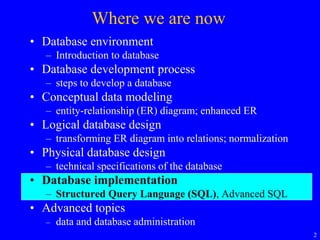
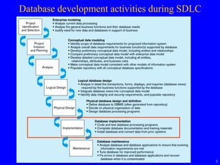
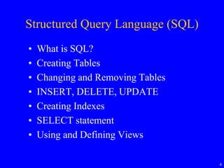
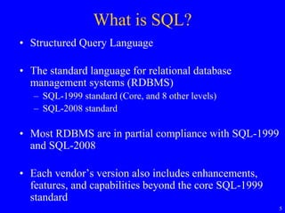
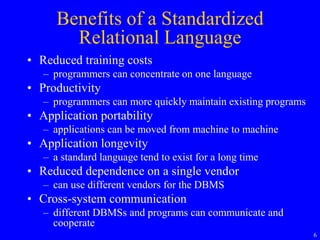
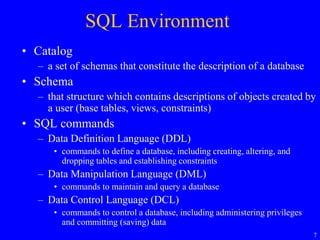
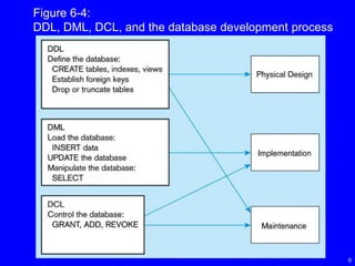
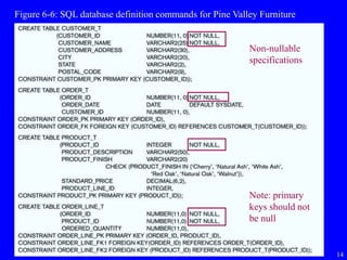
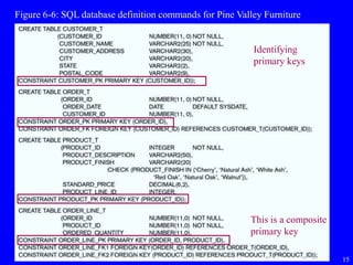
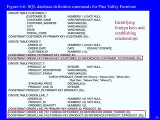
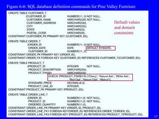
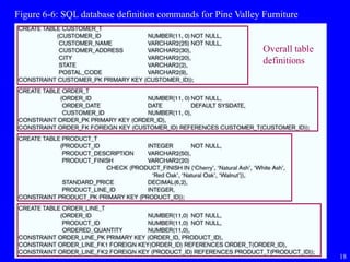
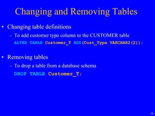
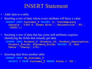
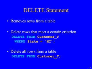
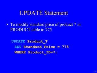
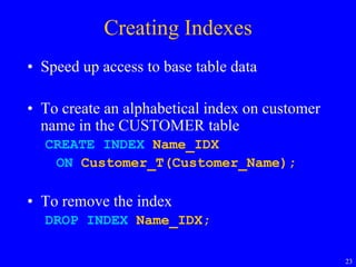
This document discusses Structured Query Language (SQL) and its role in relational database management systems. It covers: 1) SQL allows for standardized database access, reducing training costs and increasing application portability. 2) SQL commands include data definition language (DDL) to define schemas, data manipulation language (DML) to query and modify data, and data control language (DCL) to manage privileges. 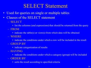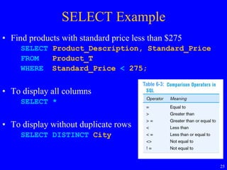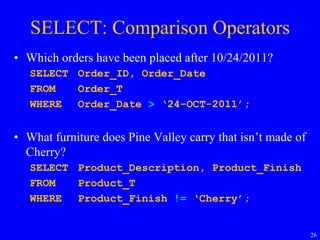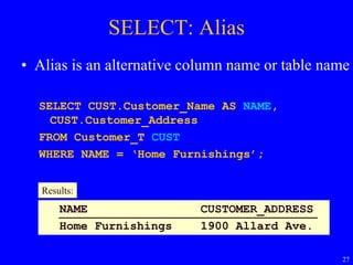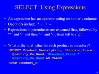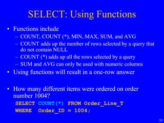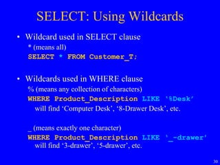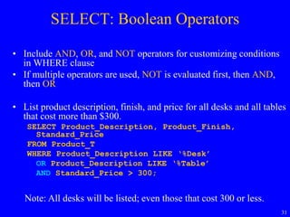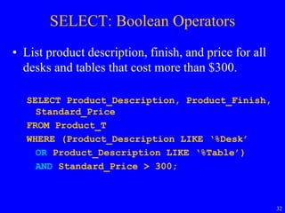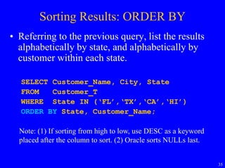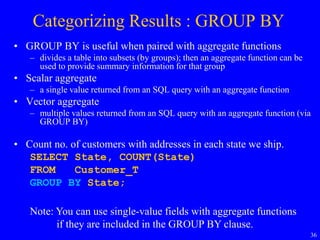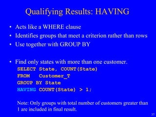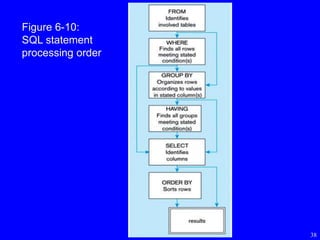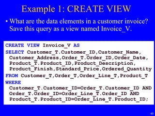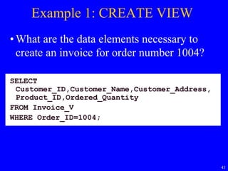3) The SELECT statement is used to query tables, allowing the use of functions, expressions, wildcards, and clauses like WHERE, GROUP BY, HAVING, and ORDER BY.

1. Lecture 7:
Structured Query Language (SQL)
ISOM3260, Spring 2014

2. 2
Where we are now
• Database environment
– Introduction to database
• Database development process
– steps to develop a database
• Conceptual data modeling
– entity-relationship (ER) diagram; enhanced ER
• Logical database design
– transforming ER diagram into relations; normalization
• Physical database design
– technical specifications of the database
• Database implementation
– Structured Query Language (SQL), Advanced SQL
• Advanced topics
– data and database administration

3. 3
Database development activities during SDLC

4. 4
Structured Query Language (SQL)
• What is SQL?
• Creating Tables
• Changing and Removing Tables
• INSERT, DELETE, UPDATE
• Creating Indexes
• SELECT statement
• Using and Defining Views

5. 5
What is SQL?
• Structured Query Language
• The standard language for relational database
management systems (RDBMS)
– SQL-1999 standard (Core, and 8 other levels)
– SQL-2008 standard
• Most RDBMS are in partial compliance with SQL-1999
and SQL-2008
• Each vendor’s version also includes enhancements,
features, and capabilities beyond the core SQL-1999
standard

6. 6
Benefits of a Standardized
Relational Language
• Reduced training costs
– programmers can concentrate on one language
• Productivity
– programmers can more quickly maintain existing programs
• Application portability
– applications can be moved from machine to machine
• Application longevity
– a standard language tend to exist for a long time
• Reduced dependence on a single vendor
– can use different vendors for the DBMS
• Cross-system communication
– different DBMSs and programs can communicate and
cooperate

7. 7
SQL Environment
• Catalog
– a set of schemas that constitute the description of a database
• Schema
– that structure which contains descriptions of objects created by
a user (base tables, views, constraints)
• SQL commands
– Data Definition Language (DDL)
• commands to define a database, including creating, altering, and
dropping tables and establishing constraints
– Data Manipulation Language (DML)
• commands to maintain and query a database
– Data Control Language (DCL)
• commands to control a database, including administering privileges
and committing (saving) data

8. 8
Figure 6-1:
A simplified schematic of a typical SQL environment
Describes all
user schemas

9. 9
Figure 6-4:
DDL, DML, DCL, and the database development process

10. 10
Figure 6-3: Sample Pine Valley Furniture data
Customer_T Order_T
Order_Line_T
Product_T

11. 11
Creating Tables
• Identify appropriate datatype
• Identify columns that should not accept null value
(NOT NULL)
• Identify columns that need to be unique (UNIQUE
and PRIMARY KEY)
• Identify all primary key-foreign key mates
(REFERENCES)
• Identify columns for which a default value is
desired (DEFAULT)
• Identify columns for which domain specifications
may be stated (CHECK)
• Create table using CREATE TABLE command

12. 12
Figure 6-6: SQL database definition commands for Pine Valley Furniture

13. 13
Figure 6-6: SQL database definition commands for Pine Valley Furniture
Defining
attributes and
their data types

14. 14
Figure 6-6: SQL database definition commands for Pine Valley Furniture
Non-nullable
specifications
Note: primary
keys should not
be null

15. 15
Figure 6-6: SQL database definition commands for Pine Valley Furniture
Identifying
primary keys
This is a composite
primary key

16. 16
Figure 6-6: SQL database definition commands for Pine Valley Furniture
Identifying
foreign keys and
establishing
relationships

17. 17
Figure 6-6: SQL database definition commands for Pine Valley Furniture
Default values
and domain
constraints

18. 18
Figure 6-6: SQL database definition commands for Pine Valley Furniture
Overall table
definitions

19. 19
Changing and Removing Tables
• Changing table definitions
– To add customer type column to the CUSTOMER table
ALTER TABLE Customer_T ADD(Cust_Type VARCHAR2(2));
• Removing tables
– To drop a table from a database schema
DROP TABLE Customer_T;

20. 20
INSERT Statement
• Adds data to a table
• Inserting a row of data where every attribute will have a value
INSERT INTO Customer_T VALUES (1,‘Contemporary
Casuals’,‘1355 S. Himes Blvd.’,‘Gainesville’,‘FL’,
‘32601’);
• Inserting a row of data that has some null attributes requires
identifying the fields that actually get data
INSERT INTO Product_T (Product_ID, Product_Description,
Product_Finish, Standard_Price) VALUES (1,‘End
Table’,‘Cherry’,175);
• Inserting data from another table
INSERT INTO CA_Customer_T
SELECT * FROM Customer_T WHERE State = ‘CA’;

21. 21
DELETE Statement
• Removes rows from a table
• Delete rows that meet a certain criterion
DELETE FROM Customer_T
WHERE State = ‘HI’;
• Delete all rows from a table
DELETE FROM Customer_T;

22. 22
UPDATE Statement
• To modify standard price of product 7 in
PRODUCT table to 775
UPDATE Product_T
SET Standard_Price = 775
WHERE Product_ID=7;

23. 23
Creating Indexes
• Speed up access to base table data
• To create an alphabetical index on customer
name in the CUSTOMER table
CREATE INDEX Name_IDX
ON Customer_T(Customer_Name);
• To remove the index
DROP INDEX Name_IDX;

24. 24
SELECT Statement
• Used for queries on single or multiple tables
• Clauses of the SELECT statement
– SELECT
• list the columns (and expressions) that should be returned from the query
– FROM
• indicate the table(s) or view(s) from which data will be obtained
– WHERE
• indicate the conditions under which a row will be included in the result
– GROUP BY
• indicate categorization of results
– HAVING
• indicate the conditions under which a category (group) will be included
– ORDER BY
• sorts the result according to specified criteria

25. 25
SELECT Example
• Find products with standard price less than $275
SELECT Product_Description, Standard_Price
FROM Product_T
WHERE Standard_Price < 275;
• To display all columns
SELECT *
• To display without duplicate rows
SELECT DISTINCT City
Table 6-3:

26. 26
SELECT: Comparison Operators
• Which orders have been placed after 10/24/2011?
SELECT Order_ID, Order_Date
FROM Order_T
WHERE Order_Date > ‘24-OCT-2011’;
• What furniture does Pine Valley carry that isn’t made of
Cherry?
SELECT Product_Description, Product_Finish
FROM Product_T
WHERE Product_Finish != ‘Cherry’;

27. 27
SELECT: Alias
• Alias is an alternative column name or table name
SELECT CUST.Customer_Name AS NAME,
CUST.Customer_Address
FROM Customer_T CUST
WHERE NAME = ‘Home Furnishings’;
NAME CUSTOMER_ADDRESS
Home Furnishings 1900 Allard Ave.
Results:

28. 28
SELECT: Using Expressions
• An expression has an operator acting on numeric columns
• Operators include: *, / , +, –
• Expressions in parentheses are executed first, followed by
‘*’ and ‘/’ and then ‘+’ and ‘-’, from left to right
• What is the total value for each product in inventory?
SELECT Product_Description, Standard_Price,
Quantity_On_Hand, Standard_Price *
Quantity_On_Hand AS VALUE
FROM Product_T;

29. 29
SELECT: Using Functions
• Functions include
– COUNT, COUNT (*), MIN, MAX, SUM, and AVG
– COUNT adds up the number of rows selected by a query that
do not contain NULL
– COUNT (*) adds up all the rows selected by a query
– SUM and AVG can only be used with numeric columns
• Using functions will result in a one-row answer
• How many different items were ordered on order
number 1004?
SELECT COUNT(*) FROM Order_Line_T
WHERE Order_ID = 1004;

30. 30
SELECT: Using Wildcards
• Wildcard used in SELECT clause
* (means all)
SELECT * FROM Customer_T;
• Wildcards used in WHERE clause
% (means any collection of characters)
WHERE Product_Description LIKE ‘%Desk’
will find ‘Computer Desk’, ‘8-Drawer Desk’, etc.
_ (means exactly one character)
WHERE Product_Description LIKE ‘_-drawer’
will find ‘3-drawer’, ‘5-drawer’, etc.

31. 31
SELECT: Boolean Operators
• Include AND, OR, and NOT operators for customizing conditions
in WHERE clause
• If multiple operators are used, NOT is evaluated first, then AND,
then OR
• List product description, finish, and price for all desks and all tables
that cost more than $300.
SELECT Product_Description, Product_Finish,
Standard_Price
FROM Product_T
WHERE Product_Description LIKE ‘%Desk’
OR Product_Description LIKE ‘%Table’
AND Standard_Price > 300;
Note: All desks will be listed; even those that cost 300 or less.

32. 32
SELECT: Boolean Operators
• List product description, finish, and price for all
desks and tables that cost more than $300.
SELECT Product_Description, Product_Finish,
Standard_Price
FROM Product_T
WHERE (Product_Description LIKE ‘%Desk’
OR Product_Description LIKE ‘%Table’)
AND Standard_Price > 300;

33. 33
SELECT: Ranges
• Which products have a price between $200 and
$300?
SELECT Product_Description, Standard_Price
FROM Product_T
WHERE Standard_Price > 199 AND
Standard_Price < 301;
SELECT Product_Description, Standard_Price
FROM Product_T
WHERE Standard_Price BETWEEN 200 AND 300;

34. 34
SELECT: IN and NOT IN Lists
• List all customers who live in warmer states.
SELECT Customer_Name, City, State
FROM Customer_T
WHERE State IN (‘FL’,‘TX’,‘CA’,‘HI’);
Note: The IN operator in this example allows you to include
rows whose STATE value is either FL, TX, CA, or HI. It is more
efficient than separate OR conditions.

35. 35
Sorting Results: ORDER BY
• Referring to the previous query, list the results
alphabetically by state, and alphabetically by
customer within each state.
SELECT Customer_Name, City, State
FROM Customer_T
WHERE State IN (‘FL’,‘TX’,‘CA’,‘HI’)
ORDER BY State, Customer_Name;
Note: (1) If sorting from high to low, use DESC as a keyword
placed after the column to sort. (2) Oracle sorts NULLs last.

36. 36
Categorizing Results : GROUP BY
• GROUP BY is useful when paired with aggregate functions
– divides a table into subsets (by groups); then an aggregate function can be
used to provide summary information for that group
• Scalar aggregate
– a single value returned from an SQL query with an aggregate function
• Vector aggregate
– multiple values returned from an SQL query with an aggregate function (via
GROUP BY)
• Count no. of customers with addresses in each state we ship.
SELECT State, COUNT(State)
FROM Customer_T
GROUP BY State;
Note: You can use single-value fields with aggregate functions
if they are included in the GROUP BY clause.

37. 37
Qualifying Results: HAVING
• Acts like a WHERE clause
• Identifies groups that meet a criterion rather than rows
• Use together with GROUP BY
• Find only states with more than one customer.
SELECT State, COUNT(State)
FROM Customer_T
GROUP BY State
HAVING COUNT(State) > 1;
Note: Only groups with total number of customers greater than
1 are included in final result.

38. 38
Figure 6-10:
SQL statement
processing order

39. 39
Using and Defining Views
• Base table
– a table containing the raw data
• Dynamic view
– a “virtual table” created dynamically upon request by a user
– no data actually stored; instead data from base table made
available to user
– based on SELECT statement on base tables or other views
• Advantages of views
– simplify query commands
– provide data security
– enhance programming productivity
• CREATE VIEW command

40. 40
Example 1: CREATE VIEW
• What are the data elements in a customer invoice?
Save this query as a view named Invoice_V.
CREATE VIEW Invoice_V AS
SELECT Customer_T.Customer_ID,Customer_Name,
Customer_Address,Order_T.Order_ID,Order_Date,
Product_T.Product_ID,Product_Description,
Product_Finish,Standard_Price,Ordered_Quantity
FROM Customer_T,Order_T,Order_Line_T,Product_T
WHERE
Customer_T.Customer_ID=Order_T.Customer_ID AND
Order_T.Order_ID=Order_Line_T.Order_ID AND
Product_T.Product_ID=Order_Line_T.Product_ID;

41. 41
Example 1: CREATE VIEW
• What are the data elements necessary to
create an invoice for order number 1004?
SELECT
Customer_ID,Customer_Name,Customer_Address,
Product_ID,Ordered_Quantity
FROM Invoice_V
WHERE Order_ID=1004;

42. 42
Using and Defining Views
• Some people suggest creating a view for every
base table, even if that view is identical to the
base table
• Greater programming productivity
– If the programs use the CUSTOMER_T and
CUSTOMER_T is renormalized into 2 tables, then
all the programs have to be modified
– If the programs use a view on the CUSTOMER_T
and CUSTOMER_T is renormalized into 2 tables,
then only the view has to be recreated

43. 43
Review Questions
• What are the benefits of SQL?
• What is the SQL environment?
• How to CREATE, ALTER, and DROP tables?
• How to INSERT, UPDATE, and DELETE rows
from tables?
• How to CREATE and DROP indexes?
• How to retrieve data using SELECT statement?
• What are views?